Understanding VGGNet - Very Deep Convolutional Networks for Large-Scale Image Recognition
Posted on 2/16/2025
After having analyzed and implemented AlexNet, it’s time to move forward and study the work presented by Karen Simonyan and Andrew Zisserman in their 2014 paper Very Deep Convolutional Networks for Large-Scale Image Recognition. The network they created is commonly referred to as VGGNet, as the authors were part of the Visual Geometry Group (VGG) at the University of Oxford.
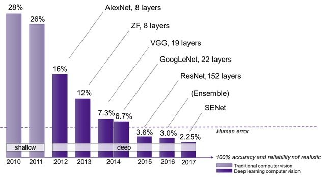
VGGNet was developed, like AlexNet, for the 2014 ILSVRC competition. Even though it did not win the 2014 ILSVRC classification competition, which was awarded to GoogLeNet, VGGNet won the localization task and has become relevant due to its depth, simple design, and performance. Furthermore, VGGNet became the foundation for other applications such as object detection, image segmentation, and style transfer.
The authors created a set of top-performing ConvNets that built on previous results and observations, such as:
- In 2012, Krizhevsky et al. noted that the depth of the network is a crucial parameter and that better results could be obtained by simply making the network larger.
- The 2013 ILSVRC winner used a smaller receptive window size and a smaller stride on the first convolutional layer.
- Sermanet et al.1 and Howard had shown performance improvements when training the networks over the whole image at multiple scales, which, as we will see later, requires architectural modifications since, up to this point, fixed-size input images were used.
VggNet Architecture
An important difference between this network and previous ones (e.g., AlexNet) was the complexity of the kernels used in the convolutional layers. Previous networks used large kernels in the first layers (11 channels for AlexNet), which progressively became smaller. The approach for VGGNet was different and much simpler: they used a 3x3 kernel for all convolutional layers in the network. The reason for using this size is that a 3x3 filter is the smallest size that allows for capturing the notion of left, right, up, down, and center. The use of small kernels was not pioneered by VGGNet, as they had been previously employed 2, but never for such deep networks.
According to the authors, using smaller kernels has some advantages:
- Using smaller kernels means that the receptive field (which is the region of the input image that a neuron in the network can see) of each individual layer is also smaller. Therefore, we require more layers to reach the same (larger) receptive field that the first layer had in previous networks. This adds more non-linearities, which allows for creating more complex decision functions.
- The number of parameters is reduced. The example they used in the paper is that three layers of 3x3 filters have parameters, while a 7x7 filter, which has the same receptive field, requires , 81% more parameters. This will allow for creating deeper networks while keeping the number of parameters similar to other shallower nets.
The authors primarily investigated the effect of depth on network accuracy by testing different configurations, ranging from 11 to 19 layers, all based on the same principles. Some of the configurations explored involved slightly different architectures, namely:
- A-LRN: They experimented with the use of Local Response Normalization (LRN) following the path (and settings) of AlexNet. However, they observed that using LRN did not improve accuracy and increased memory consumption and computation time. Therefore, they decided not to use it.
- C: Although 1x1 convolutions can be used to change the dimensionality of the filter space, in VGGNet they were added to increase the non-linearity of the decision function without modifying the receptive field 3.
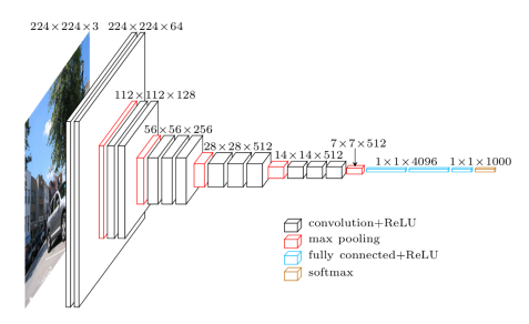
All configurations are composed of 5 convolutional blocks, each followed by a max-pooling layer, and end with a three-layer fully connected classification block. The number of kernel channels is kept constant within each convolutional block, starting at 64 in the first layer and doubling with each subsequent convolutional block until reaching 512. The main difference between the different configurations is the number of convolutional layers in each convolutional block.
The table below contains all the VGGNet configurations explored in the original paper.
| A | A-LRN | B | C | D | E | |
|---|---|---|---|---|---|---|
| Layers | 11 | 11 | 13 | 16 | 16 | 19 |
| Weights (mill.) | 133 | 133 | 133 | 134 | 138 | 144 |
| Conv 1 | conv3-64 | conv3-64 | conv3-64 | conv3-64 | conv3-64 | conv3-64 |
| LRN | conv3-64 | conv3-64 | conv3-64 | conv3-64 | ||
| Maxpool | ||||||
| Conv 2 | conv3-128 | conv3-128 | conv3-128 | conv3-128 | conv3-128 | conv3-128 |
| conv3-128 | conv3-128 | conv3-128 | conv3-128 | |||
| Maxpool | ||||||
| Conv 3 | conv3-256 | conv3-256 | conv3-256 | conv3-256 | conv3-256 | conv3-256 |
| conv3-256 | conv3-256 | conv3-256 | conv3-256 | conv3-256 | conv3-256 | |
| conv1-256 | conv3-256 | conv3-256 | ||||
| Maxpool | ||||||
| Conv 4 | conv3-512 | conv3-512 | conv3-512 | conv3-512 | conv3-512 | conv3-512 |
| conv3-512 | conv3-512 | conv3-512 | conv3-512 | conv3-512 | conv3-512 | |
| conv1-512 | conv3-512 | conv3-512 | ||||
| Maxpool | ||||||
| Conv 5 | conv3-512 | conv3-512 | conv3-512 | conv3-512 | conv3-512 | conv3-512 |
| conv3-512 | conv3-512 | conv3-512 | conv3-512 | conv3-512 | conv3-512 | |
| conv1-512 | conv3-512 | conv3-512 | ||||
| Maxpool | ||||||
| FC-4096 | ||||||
| FC-4096 | ||||||
| FC-1000 | ||||||
| Softmax | ||||||
These configurations are composed of the following common blocks, reused across all configurations and convolutional layers:
- 224x224 RGB images as input.
- 3x3 convolutional kernels with a stride of 1 and padding of 1 (so that the spatial resolution remains the same after the convolution), followed by a ReLU non-linearity.
- Max-pooling of size 2x2 with a stride of 2. Remember that AlexNet used 2x2 overlapping max-pooling.
- A classification block at the end consisting of three fully connected layers:
- Fully connected layer with 25088 inputs, 4096 neurons (like in AlexNet), dropout applied with a probability of 0.5, and ReLU activation function.
- Fully connected layer with 4096 inputs, 4096 neurons, dropout applied with a probability of 0.5, and ReLU activation function.
- Fully connected layer with 4096 inputs, 1000 units, and a Softmax activation function.
These networks contain around 140 million parameters, more than twice the size of AlexNet. Therefore, some of the concerns expressed by Krizhevsky and Sutskever, such as data augmentation to avoid overfitting, network initialization, and computational times, will be even more relevant here.
VGGNet is similar to GoogLeNet in that both are very deep CNNs with small convolution filters. However, the GoogLeNet architecture was more complex, with feature maps that reduced more in the first layers.
Data Processing and Augmentation
The data pre-processing employed for VGGNet is exactly the same as that for AlexNet: the entire variable-size dataset is rescaled so that the shorter side has a length of 256 pixels, and then the mean RGB value computed per pixel per channel for the entire dataset (1.2 million images!) is subtracted. This is done to center the input values around zero to improve convergence.
As mentioned in the previous section, VGGNet is a large convolutional network with around 140 million parameters to adjust. Therefore, having good data augmentation techniques will be essential to avoid overfitting. Some of the data augmentation techniques used for AlexNet were also used for VGGNet, such as PCA color augmentation with the same settings and a 50% chance of horizontally flipping an image. However, one new technique was added. Remember how in AlexNet we randomly cropped 227x227 square images from the original 256x256? For VGGNet, two different approaches were used for setting the training scale:
- Fixed image scale: The original input image is rescaled to a new size, from which 224x224 random crops are extracted. The authors used 256 (the same as in AlexNet) and 384 as fixed values. It is worth mentioning that the network with the original input size of 384 was not trained from scratch; rather, it was initialized with pre-trained weights from previous iterations, and a learning rate of 0.001 was used.
- Sampling input crops from multi-scale images: The second approach consisted of rescaling each image to a size between 256 and 512, from which the 224 crop is taken. According to the authors, this scale jittering is beneficial for detecting objects of different sizes, although it’s also true that there are objects of varying sizes in the different training images of each class. As in the previous case, the model was not trained from scratch, as they used the weights from the 384 input image case.
Learning
The learning settings used to train VGGNet were almost identical to those of AlexNet.
The network was trained by optimizing the multinomial logistic regression (maximum entropy) using stochastic gradient descent with a batch size of 256, momentum of 0.9, and weight decay of 0.0005.
The learning rate was set to 0.01 and decreased by a factor of 10 when the validation accuracy stopped improving.
A correct initialization of the network is really important to avoid vanishing or exploding gradients, which deep neural networks tend to suffer from. The original paper proposes two alternatives to initialize the different VGGNets:
- Initialize the most shallow VGGNet (configuration A) and train using randomly initialized parameters. The weights are drawn from a normal distribution with zero mean and a variance of 0.01, and the biases are set to 0. Note the different initialization with respect to AlexNet, in which the biases of some layers are set to 1 to avoid dying neurons. In order to train deeper configurations, the (trained) parameters of configuration A are used to initialize the first four convolutional layers and the fully connected block, while keeping the initial learning rate.
- Random initialization using the procedure of Glorot and Bengio 4, independently of the configuration. This initialization is normally also called Xavier initialization, after Xavier Glorot.
The implementation of the code used the C++ Caffe toolbox, but with important modifications to enable the use of multiple GPUs simultaneously and to evaluate uncropped images at multiple scales.
The training was conducted using 4 NVIDIA Titan Black GPUs with 6GB of memory and took around 2-3 weeks per network. The paper mentions that (for an unknown configuration) it took 74 epochs to train, during which the learning rate was reduced three times. This is less than AlexNet, which might be caused by the pre-initialization of some of the weights.
Testing
The strategy for testing VGGNet is similar to that of Sermanet et al. 5, and allows for testing (square) images of different sizes by applying the network densely over the test image. This can be achieved by converting the fully connected layers into convolutional layers. For instance, in VGGNet, the first fully connected layer has 4096 neurons with an input of shape 7x7x512. This fully connected layer can be converted into 4096 convolutional kernels of size 7x7x512, which will produce an output of 1x1x4096. We can also verify that both have the same number of parameters:
- FC1 parameters: (input size) 7x7x512x4096 (node number) + 4096 (bias for each node)
- New Conv1 parameters: (kernel size) 7x7x512x4096 (kernels) + 4096 (bias for each kernel)
In order to convert the fully connected layers into convolutional layers, we will need to reshape each of the weight matrices in the following way:
- First FC -> 4096 7x7x512 kernels.
- Second FC -> 4096 1x1x4096 kernels.
- Third FC -> 1000 1x1x4096 kernels.
Note that when the input image is 224x224, this transformation will lead to a 1x1x1000 tensor, which will be the input to the Softmax function. However, when the input size is larger than 224, the output of the new third convolutional layer will be (>1)x(>1)x1000. In order to obtain a vector with class scores, we will sum-pool (or average pool) along these dimensions to reduce the shape to 1x1x1000.
This method of evaluating images at test time is called dense evaluation in the original paper, and removes the need to create multiple crops during test time, as was done for AlexNet. The paper analyzed results for all configurations when testing using a single scale (256 or 384) and multiple scales [224, 384, 512], with the results of the three scales averaged.
The authors also augment by horizontally flipping the images and averaging the solution of the original and flipped images to obtain the final scores for the image.
Simonyan and Zisserman also studied the effect of using multiple cropping at evaluation time. They used the same approach as GoogLeNet 6, using 50 crops per scale (5x5 grid with 2 flips) or 150 crops over 3 scales. Nonetheless, they acknowledge that the increased computation time of so many crops does not justify the potential gains in accuracy.
Results and Conclusions
The classification performance of the network is evaluated using two measures: top-1 and top-5 error. Top-1 refers to whether the correct class is the one with the maximum probability, and top-5 refers to whether the correct class is within the five classes with the largest probabilities.
From the single-scale evaluation (either 256 or 384), the authors drew the following conclusions:
- Local Response Normalization (A-LRN) does not improve the model compared to the non-normalized configuration A.
- The classification error decreases with increased ConvNet depth.
- The configurations with 1x1 convolutional layers perform worse than the equivalent configurations with 3x3 kernels. They conclude that even though 1x1 convolutions help (as C performs better than B), it is important to capture the spatial context by using convolutional filters (D performs better than C).
- The error rate of the VGGNet architecture saturates when depth reaches 19 layers, but they note that larger models might be beneficial for larger datasets.
- They confirmed that a deep net with small filters outperforms a shallow net with larger filters by replacing the pairs of 3x3 kernels of configuration B with a single 5x5 filter.
- Scale jittering at training time leads to significantly better results than training on images with a fixed smallest side, even when using a single scale at test time. This confirmed how this technique can help capture multi-scale image statistics.
- Scale jittering at test time leads to better performance.
The authors also compared the performance of configurations D and E when using different evaluation techniques, namely dense evaluation, multi-crop, and both. They observed that multiple crops performed slightly better than dense evaluation and that using both provided the best results. They concluded that these two approaches are complementary because they treat the convolution boundary conditions differently.
| VggNet Config | Evaluation method | top-1 val. error (%) | top-5 val. error (%) |
|---|---|---|---|
| D - Vgg16 | dense | 24.8 | 7.5 |
| multi-crop | 24.6 | 7.3 | |
| multi-crop & dense | 24.4 | 7.2 | |
| E - Vgg19 | dense | 24.8 | 7.5 |
| multi-crop | 24.6 | 7.4 | |
| multi-crop & dense | 24.4 | 7.1 |
The table above contains the top-1 and top-5 validation error rates for VGG16 and VGG19 using different evaluation techniques. It can be seen that the differences between them are quite small, even though configuration E (VGG19) contains 6 million more parameters, and the multi-crop evaluation requires 50 or 150 (multi-crop + dense) images compared to 3 with dense evaluation. For all of this, using VGG16 with dense evaluation might be a good compromise between accuracy and computational time/complexity.
As is typically done, the authors also used ConvNet fusion, combining the outputs of several models by averaging their predictions, to improve overall performance. With this technique, they achieved a top-5 error rate of 6.8% using combined dense evaluation and multi-crop. In contrast, the best single model achieved a 7.1% top-5 error rate.
The table below is presented in the paper and compares VGGNet with the state-of-the-art models at that time. VGGNet placed 2nd, just after GoogLeNet, when using ConvNet fusion, and 1st in single-model accuracy.
| Method | top-1 val. error (%) | top-5 val. error (%) | top-5 test error (%) | |
|---|---|---|---|---|
| VGG (2 nets, multi-crop & dense eval.) | 23.7 | 6.8 | 6.8 | |
| VGG (1 net, multi-crop & dense eval.) | 24.4 | 7.1 | 7.0 | |
| VGG (ILSVRC submission, 7 nets, dense eval.) | 24.7 | 7.5 | 7.3 | |
| GoogLeNet6 (1 net) | - | 7.9 | 7.9 | |
| GoogLeNet6 (7 nets) | - | 6.7 | 6.7 | |
| MSRA7 (11 nets) | - | - | 8.1 | |
| MSRA7 (1 net) | 27.9 | 9.1 | 9.1 | |
| Clarifai8 (multiple nets) | - | - | 11.7 | |
| Clarifai8 (1 net) | - | - | 12.5 | |
| Zeiler & Fergus9 (6 nets) | 36.0 | 14.7 | 14.8 | |
| Zeiler & Fergus9 (1 net) | 37.5 | 16.0 | 16.1 | |
| OverFeat1 (7 nets) | 34.0 | 13.2 | 13.6 | |
| OverFeat1 (1 net) | 35.7 | 14.2 | - | |
| Krizhevsky et al.10(7 nets) | 38.1 | 16.4 | 16.4 | |
| Krizhevsky et al.10 (1 net) | 40.7 | 18.2 | - |
The performance of VGGNet showed the importance of depth in convolutional networks with a simple architecture, following the steps of AlexNet. The authors noted, nonetheless, that after 19 layers, the accuracy of the architecture plateaued and convergence became difficult, indicating that innovations in the architecture would be required to increase the performance of these systems. This would give rise to a new type of convolutional neural network: ResNets.
Footnotes
-
Sermanet, P. (2013). Overfeat: Integrated Recognition, Localization and Detection Using Convolutional networks. arXiv preprint arXiv:1312.6229. ↩ ↩2 ↩3
-
Ciresan, D. C., Meier, U., Masci, J., Gambardella, L. M., & Schmidhuber, J. (2011, June). Flexible, high performance convolutional neural networks for image classification. In Twenty-second international joint conference on artificial intelligence. ↩
-
Lin, M. (2013). Network in network. arXiv preprint arXiv:1312.4400. ↩
-
Glorot, X., & Bengio, Y. (2010, March). Understanding the difficulty of training deep feedforward neural networks. In Proceedings of the thirteenth international conference on artificial intelligence and statistics (pp. 249-256). JMLR Workshop and Conference Proceedings. ↩
-
Ciresan, D. C., Meier, U., Masci, J., Gambardella, L. M., & Schmidhuber, J. (2011, June). Flexible, high performance convolutional neural networks for image classification. In Twenty-second international joint conference on artificial intelligence. ↩
-
Szegedy, C., Liu, W., Jia, Y., Sermanet, P., Reed, S., Anguelov, D., … & Rabinovich, A. (2015). Going deeper with convolutions. In Proceedings of the IEEE conference on computer vision and pattern recognition (pp. 1-9). ↩ ↩2 ↩3
-
He, K., Zhang, X., Ren, S., & Sun, J. (2015). Spatial pyramid pooling in deep convolutional networks for visual recognition. IEEE transactions on pattern analysis and machine intelligence, 37(9), 1904-1916. ↩ ↩2
-
Russakovsky, Olga, Jia Deng, Hao Su, Jonathan Krause, Sanjeev Satheesh, Sean Ma, Zhiheng Huang et al. “Imagenet large scale visual recognition challenge.” International journal of computer vision 115 (2015): 211-252. ↩ ↩2
-
Zeiler, M. D., & Fergus, R. (2014). Visualizing and understanding convolutional networks. In Computer Vision–ECCV 2014: 13th European Conference, Zurich, Switzerland, September 6-12, 2014, Proceedings, Part I 13 (pp. 818-833). Springer International Publishing. ↩ ↩2
-
Krizhevsky, A., Sutskever, I., & Hinton, G. E. (2012). Imagenet classification with deep convolutional neural networks. Advances in neural information processing systems, 25. ↩ ↩2
Comments
No comments yet.