Understanding AlexNet - ImageNet Classification with Deep Convolutional Neural Networks
Posted on 1/2/2025
In this post I will explore the paper ImageNet Classification with Deep Convolutional Neural Networks by Alex Krizhevsky, Ilya Sutskever, and Geoffrey Hinton. The goal is to understand the details and rationale behind its data processing, network architecture, and learning process. This post is the first in a two-part series: in the first part, I will analyze the paper, and in the second part, we will implement—and hopefully run—the network. The network introduced in the paper is widely known as AlexNet. It was designed by Alex Krizhevsky in collaboration with Ilya Sutskever and Geoffrey Hinton, Krizhevsky’s Ph.D. advisor at the University of Toronto in 2012.
AlexNet was developed for the ImageNet Large-Scale Visual Recognition Challenge (ILSVRC) held in 2012. The ILSVRC was an annual competition that started in 2010 as part of the Pascal Visual Object Challenge and which used ImageNet as training, validation and test dataset. The story of ImageNet it’s also interesting on its own, as it was started by AI researcher Fei-Fei Li and is based on the WordNet dataset, an ontologically structured dataset of English terms created by Christiane Fellbaum. 1
The development of AlexNet marked a pivotal moment in the fields of computer vision and deep learning for several reasons:
- Prior to 2012, winning ILSVRC architectures were based on traditional machine learning methods. These approaches relied heavily on handcrafted features for image recognition and achieved limited success. For instance, the 2011 winning model had a top-5 error rate of 25.8%, and the second-best architecture in 2012 (ISI) had an error rate of 26.2%. In contrast, the deep neural network developed by Krizhevsky and Sutskever, which was one of the largest of its kind at the time, achieved a top-5 test error rate of 15.3%.
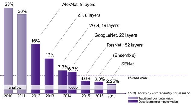
- They wrote and publicly shared a highly-optimized GPU implementation which became the standard for the following years.
- AlexNet introduced several innovative features for its time to improve performance and reduce training time. These included using ReLU as the activation function, Local Response Normalization, overlapping pooling, dropout in the hidden layers, and data augmentation techniques such as PCA color augmentation.
The Dataset
The ILSVRC 2012 dataset was a reduced version of the full ImageNet, comprising 1,000 classes with 1.2 million training images, 50,000 validation images, and 150,000 testing images. The full original database (147 GB) can be found here.
ImageNet organizes images into subfolders for each class, named using a variant of the WordNet schema (e.g., n04266014 corresponds to “space shuttle”). Each folder contains RGB images of varying resolutions. For instance, after exploring the entire dataset, I found that the largest image belongs to the class n03697007 (lumbermill, sawmill) with a size of 7056x4488 (image n03697007_27544), while the smallest one belongs to the class n07760859 (custard apple) with a size of 20x17 (image n07760859_5275).
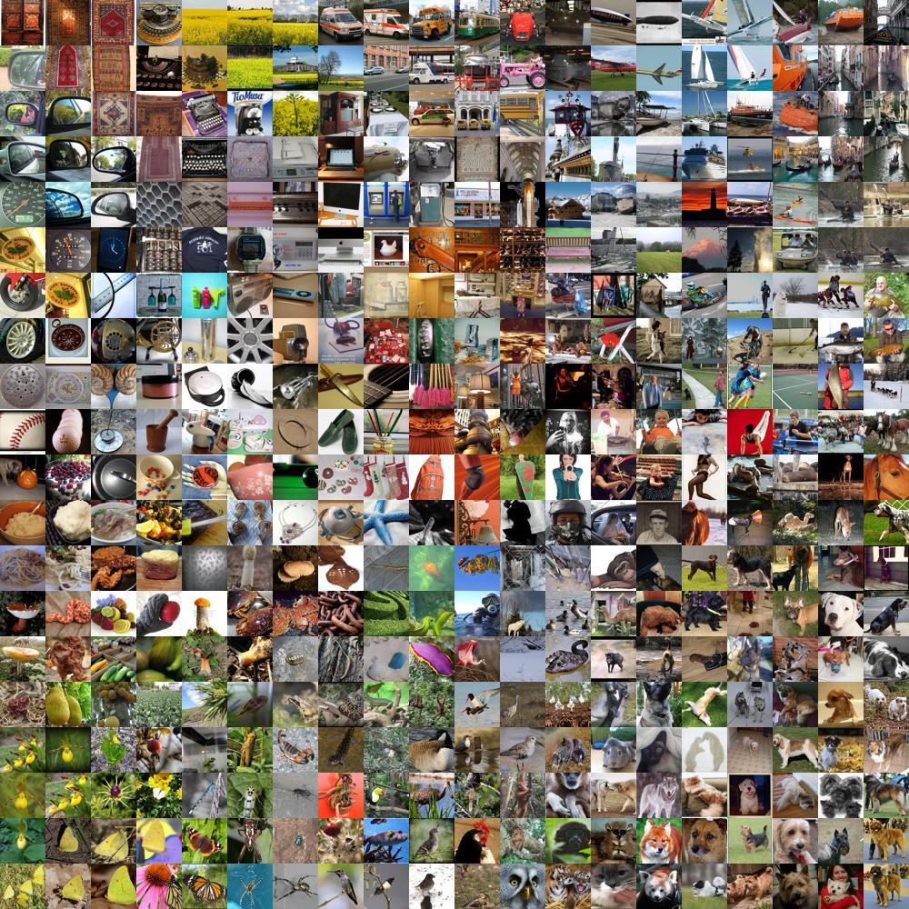
Since AlexNet requires input images to have a fixed size, the first part of the data processing consists in rescaling and cropping the images to a fixed size of 256x256 pixels. To do that, each image is rescaled so that its shorter side measures 256 pixels, and then the central 256x256 patch is cropped. In order to reduce the memory usage, we can use the resized and cropped dataset as our base training dataset. By doing this, the dataset size on disk is reduced from 147GB to 15GB, a 90% reduction!
Due to the relatively large size of the original database, alternative versions are available, such as the downsampled 32x32 version and 64x64 version. There are even reduced versions such as the tiny ImageNet dataset, that contains 100,000 images at 64x64 resolution with 200 classes, that is 500 images per class, or Imagenette, which only contains 10 easily distinguishable classes and 13,000 images.
Novel features
ReLU
The rectified linear unit (ReLU) non-linearity was first introduced by A. Householder in 1941 as a mathematical abstraction for neural networks 2 and later reintroduced by K. Fukushima in 1969 for visual feature extraction in neural networks 3.
At the time Alexnet was introduced, the most commonly used activation functions were the sigmoid, defined as , and the hyperbolic tangent (tanh), defined as . These functions are very similar except the range of the tanh function is while the sigmoid range is .

The main issue with the tanh and sigmoid activation functions is that near their asymptotes, the slope or derivative becomes very small, approaching zero. This is known as the vanishing gradient problem, caused by the saturation of the neurons. When this occurs, the network’s training slows considerably, since gradients are used during backpropagation to adjust the weights. The problem becomes even worse in deep networks where gradients at each layer are multiplied because of the chain rule. This can lead to a negligleable final gradient which makes training very slow.
On the other hand, ReLU is defined as , so if the value of the gradient will be constant, meaning that even if is very large the neurons will not saturate, which leads to faster learning. Additionally, ReLU is computationally more efficient compared to the tanh or sigmoid functions that require exponentiation.
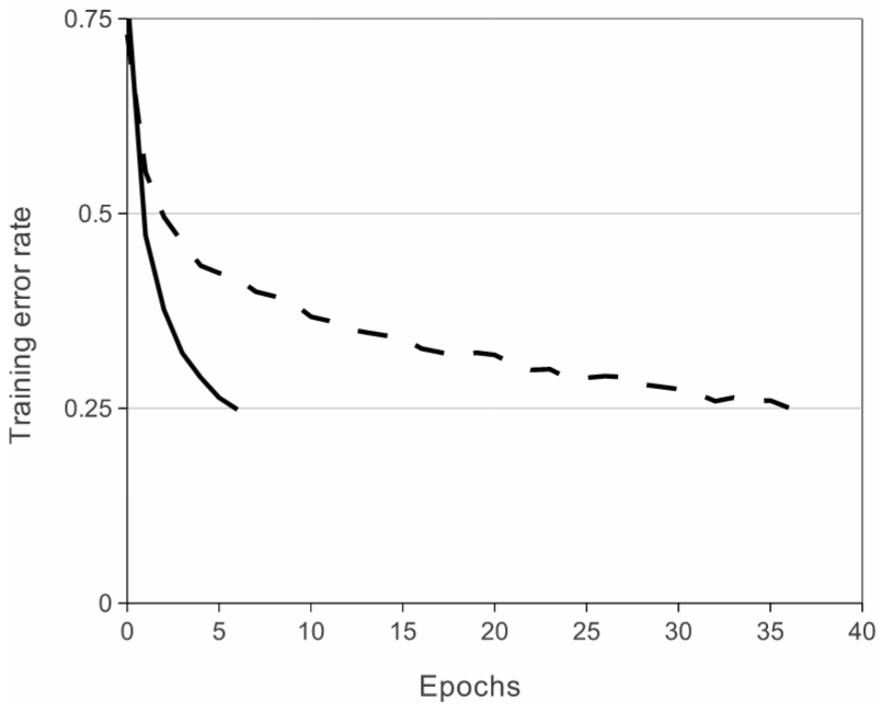
Krizhevsky and Sutskever used ReLU as their main activation function, effectively reaching 25% error rate (the best mark from the 2011 ILSVRC) six times faster compared to the same network using tanh non-linearities. Faster learning was a priority in the development of AlexNet, which is why ReLU was selected
It is important to note that there are potential problems that can arise from the use of ReLU as activation functions, the most important of which is dying neurons. This problem occurs when all inputs to the ReLU are . Since learning at each node depends on the local gradient, the local gradient for a negative will be 0 and therefore the neuron will longer update, effectively becoming a dead neuron. However, if some inputs are greater than 0, the neuron will remain active and continue learning during stochastic gradient descent. Alternative functions have been developed to address this issue, such as the LeakyReLU, where the negative domain has a small slope to prevent neurons from dying.
AlexNet demonstrated the effectiveness of ReLU in deep convolutional architectures which boosted it’s popularity. Today, ReLU is one of the most widely used activation functions in all fields where neural networks are used.
Multiple GPU training
The second novel feature of AlexNet was not so much related to its architecture, but rather to how it was run. Krizhevsky and Sutskever developed a deep convolutional network capable of running on GPUs, which allowed to train deeper and more complex networks faster than before. Their optimized GPU implementation of the 2D convolution and other operations were made publicly accessible and became a industry standard during the early years of deep learning.
The original paper discusses how they parallelized two GTX 580 GPU with 3GB using cross-GPU parallelization. By distributing the network across both GPUs, they placed half of the neurons on each and allowed communication between GPUs at certain layers. While this approach was innovative at the time, it may not be so relevant nowadays.
Local Response Normalization
This type of normalization was introduced in this paper, and is based on the idea of lateral inhibition from neurobiology. Lateral inhibition occurs when an excited neuron reduces the activity of its neighbors, creating a contrast that increases the sensory perception.
Local Response Normalization (LRN) can be applied either within the same channel or across channels. When applied within the same channel, it enhances peak responses while damping weaker ones, resulting in sharper feature maps. When applied across adjacent channels, it promotes better diversification of the feature map by creating competition among nearby channels, which leads to better features discrimination.
The LRN used in AlexNet was applied to some of the convolution layers after the ReLU activation function and it was defined as follows:
where is the activation output of a given neuron at channel , are the activation values of the same neuron at adjacent channels, and , , , are hyperparameters, whose values were determined using the validation set and fixed to (two channels before and two after the current layer), , , . Adding LRN reduced top-1 and top-5 error rates by 1.4% and 1.2% respectively.
Nowadays, LRN is less commonly used, since other techniques such as batch normalization, layer normalization or instance normalization have gained popularity.
Overlapping Pooling
Pooling layers are normally used in CNNs to downsample feature maps and increase robustness to small positional changes. In AlexNet, a max-pooling layer was added after some of the convolutional layers. Rather than setting the pooling kernel size equal to the stride, as is typically done, they chose a kernel size () larger than the stride (), resulting in overlapping pooling. This modification improved the top-1 and top-5 error rates by 0.4% and 0.3%, respectively, and reduced overfitting.
Dropout
To reduce test error, rather than combining the predictions of multiple models, which would be computationally very expensive, the authors chose to use dropout4. Dropout consists in setting the output of a hidden neuron to zero based on a given probability. These dropped neurons do not contribute to the network forward and backward passes, making the architecture different each time the network is run. This technique is intended to reduce overfitting by encouraging the network to learn more robust features. During test time the network is run using all neurons, but the outputs of each layer are scaled by a factor.
Data Processing and Augmentation
In this section, I will go into detail about the entire data processing pipeline applied to the original images, from when they are retrieved from the dataset to the moment they are fed into the network. Some of these processes occur at the beginning and involve simply transforming the images from the database into the correct format:
- Rescaling the variable-size image so that the shorter side has a length of 256 pixels, and then cropping out the central 256x256 patch from the resulting image.
- The 256x256 squared images are then normalized by subtracting the mean activity over the training set from each pixel. In other words, for every pixel the mean is computed separately for each position and channel. After the mean is subtracted, some pixels will have negative values. Don’t panic—while this doesn’t have any meaning in terms of pixel representation, it is numerically correct and helps speed up learning, as the gradients will act more uniformly across each channel. Later in testing the same mean substraction will be applied to test images.
Another popular alternative is to substract the per-channel mean, which is commonly used because it doesn’t require all images to be the same size.
Even with 1.2 million images in the dataset, it showed to be insufficient to learn the 60 million parameters without considerable overfitting. To address this, some data augmentation methods were employed to artificially expand the dataset:
- During the training phase, the network was fed with 227x227 images randomly cropped from the 256x256 original images.
- Images are also horizontally flipped with a 50% probability.
- PCA Color Augmentation, also called Fancy PCA, modifies the intensities of the RGB channels along the natural variations of the images, denoted by the principal components of the pixel colors5. The process begins by flattening the RGB image into a matrix of shape () where is the number of pixels per channel. The idea is to normalize them between and compute PCA on the datapoints by computing the covariance and its associated eigenvalues and eigenvectors . Then, a correction is added to each RGB channel using the formula below, where is a random variable drawn from a normal distribution with zero mean and 0.1 standard deviation. Note that the correction must be scaled to the integer range of from the original float range and added to the orginal image.
Network Architecture
The AlexNet architecture consists of eight layers, five of which are convolutional, and the last three are fully connected. Due to the implementation across two parallel GPUs, the original network had certain peculiarities regarding the points at which the two parts communicate. This choice was more influenced by computational limitations at the time rather than actual performance. For this reason, the architecture details specific to the two-part setup will be written in italics.

The input to the network is a 224x224 RGB image, which is randomly cropped from the original 256x256 image. The AlexNet architecture consists of the following layers:
- Convolutional layer with 224x224x3 input image, 96 kernels of size 11x11, stride of 4 and ReLU activation function. The output of this first convolution operation has a shape of 54x54x96, however, the original paper states that the output shape should be 55x55x96, which means there’s a discrepancy between the input and output size stated. This issue is something that has been pointed out by many. To resolve this inconsistency, I will assume the input shape is actually 227x227x3 and NOT 224x224x3, in order to keep the rest of the architecture as in the paper. This discrepancy in the input dimensions was also pointed out by Andrej Karpathy, the former head of computer vision at Tesla, who confirmed the input shape must have been 227x227x3. After the convolutional, the output is normalized using Local Response Normalization (LRN) and downsampled via max-pooling with kernel size 3 and stride 2, resulting in an output shape of 27x27x96 6. The 96 kernels are separated into two groups of 48.
- Convolutional layer with 27x27x96 input, 256 kernels of size 5x5, stride of 1 and ReLU activation function. Note that the output shape of this convolution would be 23x23x256 and from the illustration in the original paper we see that the output size must be 27x27x256. This means that a padding of 2 was used in order to preserve the input and output shape the equal. This is not something explicitly mentioned in the paper, and thus it’s easy to overlook. The output was normalized using LRN, followed by a max-pool with size 3 and stride 2. The output shape is 13x13x256. The 2 GPU implementation uses two 5x5x27 kernels, each exclusively connected to the first layer within its respective GPU (see paper illustration for more clarity).
- Convolutional layer with 13x13x256 input, 384 kernels of size 3x3, stride of 1 and ReLU activation function. A padding of 1 is applied to preserve the input dimensions, although this detail is not explicitly mentioned in the paper. The output shape is 13x13x384. The kernels in this layer are connected to all feature maps from the second layer.
- Convolutional layer with 13x13x384 input, 384 kernels of size 3x3, stride of 1, padding of 1, and ReLU activation function. The output shape is 13x13x384. The kernels in this layer are only connected to the feature maps on the same GPU from the previous layer.
- Convolutional layer with 13x13x384 input, 256 kernels of size 3x3, stride of 1, padding of 1, and ReLU activation function. The output shape is 13x13x256. The output was then normalized using LRN, followed by a max-pool operation with a kernel size of 3 and a stride of 2. The resulting output shape is 6x6x256. The kernels in this layer are only connected to the feature maps on the same GPU from the previous layer.
- Fully connected layer with 9216 input, 4096 units, dropout applied with a probability of 0.5, and ReLU activation function. All fully connected layers are also fully connected across GPUs.
- Fully connected layer with 4096 input, 4096 units, dropout applied with a probability of 0.5, and ReLU activation function.
- Fully connected layer with 4096 input, 1000 units, and Softmax activation function.
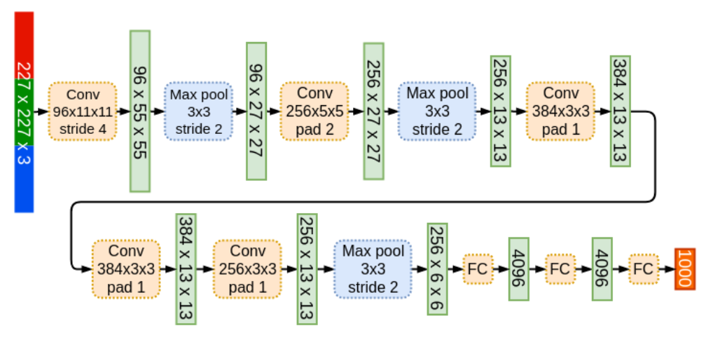
Overall, the networks contains around 60 million parameters, but over 90% of them are located in the last three fully connected layers. This can help us make an idea of how efficient in terms of learning parameters convolution layers are. The table below (obtained from source) contains a breakdown of the number of parameters (both weights and biases) for for each of the layers in AlexNet.
| Layer Name | Tensor Size | Weights | Biases | Parameters |
|---|---|---|---|---|
| Input Image | 227x227x3 | 0 | 0 | 0 |
| Conv-1 | 55x55x96 | 34,848 | 96 | 34,944 |
| MaxPool-1 | 27x27x96 | 0 | 0 | 0 |
| Conv-2 | 27x27x256 | 614,400 | 256 | 614,656 |
| MaxPool-2 | 13x13x256 | 0 | 0 | 0 |
| Conv-3 | 13x13x384 | 884,736 | 384 | 885,120 |
| Conv-4 | 13x13x384 | 1,327,104 | 384 | 1,327,488 |
| Conv-5 | 13x13x256 | 884,736 | 256 | 884,992 |
| MaxPool-3 | 6x6x256 | 0 | 0 | 0 |
| FC-1 | 4096x1 | 37,748,736 | 4,096 | 37,752,832 |
| FC-2 | 4096x1 | 16,777,216 | 4,096 | 16,781,312 |
| FC-3 | 1000x1 | 4,096,000 | 1,000 | 4,097,000 |
| Output | 1000x1 | 0 | 0 | 0 |
| Total | 62,378,344 |
Learning
The model was trained using stochastic gradient descend with a batch size of 128, momentum of 0.9, and weight decay of 0.0005.
The learning rate was the same for all layers, it was initialized at 0.01 and adjusted manually during the training. It was divided by 10 whenever the validation error rate plateaued.
The weights for each layer were initialized using a normal distribution with zero mean and standard deviation of 0.1. The biases were initialized to 1 in the second, fourth, and fifth convolutional layers in order to accelerate the learning in early stages by providing a positive input to the ReLUs and avoid dying neurons. The biases in all other layers were set to 0.
The cost function maximized during training was the multinomial logistic regression, also known as maximum entropy, which aims to maximize the log-probability of the correct labels given the predicted distributions across all training samples.
Training required 90 cycles through the entire training set, and took 5-6 days using two GTX-580 GPUs with 3GB. The learning rate had to be reduced three times during training.
Predictions at test time were made by extracting 227x227 patches (the four corners and the center) along with their horizontal reflections. The network’s final prediction was then obtained by averaging the outputs from the softmax layer for these ten patches.
Results and Conclusions
AlexNet was confronted to several editions of the ILSVRC under various configurations From these experiments, the following results were obtained:
- On ILSVRC-2010 it achieved top-1 and top-5 test set error rates of 37.5% and 17.0% outperforming the winner of that year who had recorded error rates of 47.1% and 28.2%, respectively.
- On ILSVRC-2012 different configurations were studied:
- The standard AlexNet obtained top-1 and top-5 validation error rates of 40.7% and 18.2%
- By averaging the prediction of five similar AlexNet networks, the top-1 and top-5 validation error rates achieved were 38.1% and 16.4%.
- Adding a sixth convolutional layer, training the network on the entire 2011 release (15M images and 22k categories), and fine-tuning it on the ILSVRC-2012 reulsted in error rates of 39.0% and 16.6%, respectively.
- Combining the prediction of five standard AlexNet networks and two models trained with the 2011 dataset (as in the previous point) the top-1 and top-5 validation error rates achieved were 36.7% and 15.4%, with a top-5 test error rate of 15.3%.
- On the Fall 2009 ImageNet release (8.9 million images and 10,184 categories), using a half-training half-testing split, and the AlexNet version with a sixth convolutional layer, the network obtained top-1 and top-5 error rates of 67.4% and 40.9% compared to the previous best published result of 78.1% and 60.9%.
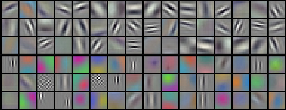
Furthermore, they studied the first-layer kernels learned by the network and found, in addition to a variety of orientations, frequencies, and blobs, a specialization between the two GPUs used during training. One GPU predominantly learned color-agnostic kernels, while the other focused on color-specific kernels. This behavior appeared to be independent of the initialization of the weights
They also measured the network’s visual understanding by computing the Euclidean distance between the activation values of the final 4096-dimensional hidden layer for pairs of images. They observed that images belonging to the same class, even if not similar in terms of pixel-level L2 distance, were still very close in this higher-dimensional space. They also suggested this similarity principles could be applied for highly efficient image retrieval methods.
Additionally, they experimented with removing convolutional hidden layers and observed a performance degradation of approximately 2% in the top-1 error rate when any middle layer was removed. From this, they concluded therefore that depth was really important and that better results could be obtained by just making the network larger and trained for longer. As we will see, this is the path that the ILSVRC winners took in the following editions.
Footnotes
-
Householder, A. S. (1941). A theory of steady-state activity in nerve-fiber networks: I. Definitions and preliminary lemmas. The bulletin of mathematical biophysics, 3, 63-69. ↩
-
Fukushima, K. (1969). Visual feature extraction by a multilayered network of analog threshold elements. IEEE Transactions on Systems Science and Cybernetics, 5(4), 322-333. ↩
-
Hinton, G. E. (2012). Improving neural networks by preventing co-adaptation of feature detectors. arXiv preprint arXiv:1207.0580. ↩
-
Bargoti, S., & Underwood, J. (2016, May). Image classification with orchard metadata. In 2016 IEEE International Conference on Robotics and Automation (ICRA) (pp. 5164-5170). IEEE. ↩
-
ConvNet output shape calculator, https://danielparicio.com/posts/convnet-calculator/ ↩
Comments
No comments yet.