Implementing Neural Style Transfer

Let’s take some time to explore one of the applications that deep convolutional neural networks enabled. In 2015, Gatys, L. A., Ecker, A. S., and Bethge, M. published A Neural Algorithm of Artistic Style, which pioneered the use of deep CNN feature layers to separate image content from style. This allowed them to formulate a simple method to transfer the style of one image onto another. In this article, I will briefly go through the formulation presented in their paper and implement it from scratch using the VGG16 weights from my previous post. I will also replicate some of the figures from the original article and provide examples of the results that can be obtained with this technique.

In the previous articles on AlexNet and VggNet, we saw that the different layers in a CNN capture information about the input image at different levels of detail. While the first layers are directly linked to the original pixel values, the deeper layers capture high-level content.

As we progress deeper into the network, feature representations become less tied to pixel-level details and reflect more of the image’s semantic content. Accordingly, the authors refer to these higher layers as the content representation. To capture style, they define a style space that harnesses texture information by computing correlations between feature-map responses. This separation of style and content is the main contribution of this work and is what allows them to manipulate each dimension independently, by applying the style (usually from a painting) of one image to the content of another to produce new, stylized outputs.

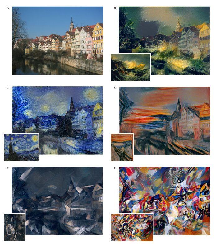
The image below shows an example from the paper in which they combine a photograph of the Neckarfront in Tübingen, Germany, with the styles of several famous paintings.

Methods

In the original paper, the authors use VGG19 as their reference convolutional network but omit its fully connected layers. Because most of the weights live in those dense layers, this cropped version is much lighter than the full network. They also replace max-pooling with average pooling, since average pooling was found to yield better results.

Below is the code snippet for the modified VGG network used in the neural style transfer.

class VggNet(torch.nn.Module):
    def __init__(self, num_classes=1000, vgg=16):
        """
        VGGNet implementation for image classification.

        Args:
            num_classes (int, optional): Number of output classes. Default is 1000 (for ImageNet).
            vgg (int, optional): VGG configuration, either 11, 13, 16 or 19 for VGG-11, VGG-16 or VGG-19. 
                                    Default is 19.
        """
        super(VggNet, self).__init__()
        self.num_classes = num_classes
        self.activation  = dict()

        if vgg not in (11, 13, 16, 19):
            raise ValueError("vgg must be 11, 13, 16, or 19")

        # Define the number of convolutional layers per block based on the VGG variant.
        # Canonical configurations:
        # VGG-11: [1, 1, 2, 2, 2]
        # VGG-13: [2, 2, 2, 2, 2]
        # VGG-16: [2, 2, 3, 3, 3]
        # VGG-19: [2, 2, 4, 4, 4]
        if vgg == 11:
            conv_counts = [1, 1, 2, 2, 2]
        elif vgg == 13:
            conv_counts = [2, 2, 2, 2, 2]
        elif vgg == 16:
            conv_counts = [2, 2, 3, 3, 3]
        else:  # vgg == 19
            conv_counts = [2, 2, 4, 4, 4]

        # Build convolutional blocks 
        self.block1 = self._create_conv_block(in_channels=3,   out_channels=64,  num_convs=conv_counts[0])
        self.block2 = self._create_conv_block(in_channels=64,  out_channels=128, num_convs=conv_counts[1])
        self.block3 = self._create_conv_block(in_channels=128, out_channels=256, num_convs=conv_counts[2])
        self.block4 = self._create_conv_block(in_channels=256, out_channels=512, num_convs=conv_counts[3])
        self.block5 = self._create_conv_block(in_channels=512, out_channels=512, num_convs=conv_counts[4])


    def _create_conv_block(self, in_channels, out_channels, num_convs):
        """
        Create a convolutional block as:
        [num_convs x (Conv2d -> ReLU)] -> MaxPool2d

        Args:
            in_channels (int): Number of input channels.
            out_channels (int): Number of output channels.
            num_convs (int): Number of convolutional layers in the block.
        Returns:
            nn.Sequential: The convolutional block.
        """
        layers = []
        for _ in range(num_convs):
            layers.append(nn.Conv2d(in_channels, out_channels, kernel_size=3, stride=1, padding=1))
            layers.append(nn.ReLU(inplace=True))
            in_channels = out_channels  # the next convolution uses out_channels as input

        layers.append(nn.AvgPool2d(kernel_size=2, stride=2)) # Modification wrt original version
        return nn.Sequential(*layers)

    
    def forward(self, x):
        x = self.block1(x)
        x = self.block2(x)
        x = self.block3(x)
        x = self.block4(x)
        x = self.block5(x)

        return x

When inputting an image to the network, this will produce a feature maps at each convolutional layer’s kernels. To recover the image encoded in a given feature map, what the authors do is to initialize a white-noise image and iteratively optimize it via gradient descent so that its feature maps match those of the original input. In practice, they save the original image’s feature responses at the desired layers, then perform gradient descent on the noise image until its feature maps are equal to the saved ones.

Let $x$ and $p$ be the original image and the generated one respectively and $P^l$ and $F^l$ their feature representation by layer $l$. Then the authors defined two losses: the content loss and the style loss and generate an input image $x$ that minimizes the total loss

• Content loss is simply given by the squared error between the content features of the synthesized image and the content image.

• Style loss: is given by the sum of many style loss from different layers

with $w_l$ the relative weight of each layer $l$ and $\mathcal{L}_{style}^l$ the squared error between style representations in layer $l$

where $N_l$ is the number of feature maps, $M_l$ is the height times the width of the feature map, and $A^l$ and $G^l$ are the style representation at layer $l$ of the original and the generated image respectively given by the Gram matrices of the feature representations.

A Gram matrix is formed by taking the inner products between every pair of feature-map vectors from a given layer. Because this operation ignores spatial positions, the resulting matrix is spatially invariant. Instead of encoding where features occur, it captures how strongly different feature channels correlate with one another.¹

![[Gram_matrix.svg]] Gram matrix construction by arranging the matrix in columns and taking the respective transpose/original scalar products to compute each elements of the matrix.

Implementation

In order to be able to implement the neural style transfer algorithm we first need a way to be able to extract the output of a particular convolution layer inside the model. Ideally, by not hard-coding what layers to save so that later one we can modify, and iterate what feature maps are used for content and style transfer. When researching on how to extract the output of hidden convolution layers, I came across this great post by Nandita Bhaskhar where she explain three ways to obtain this:

1. Lego style: consists on reconstructing a new model containing only the layers up to the one you need. This method is straightforward, but doesn’t allow for multiple outputs so I ruled it out.
2. Hack the model: In this method we modify the forward function of the model by appending the feature maps to an intermediate_outputs variable that gets returned at the end. The main problem with this method is that we have to hard-code the layers that are going to be returned, so it doesn’t allow all for the flexibility I was looking for.
3. Attach a hook: In this method a forward_hook attached to the module, when forward is called, the module, inputs and outputs are passed to the forward_hook before proceeding to the next module. The first step is to define a function to call the hook signature and store the outputs in a dictionary.

activation = {}
def getActivation(self, name):
        def hook(model, input, output):
            activation[name] = output
        return hook

I then created a method within the VggNet class to retrieve arbitrary feature layers, either for content or style, using the same convX_Y notation as in the original paper, where X refers to the convolutional block and Y to the position of the kernel within that block. The detach option is set so that the feature maps are extracted independently from the model’s computation graph, which allows us to optimize only the synthesized image later. Note that this method already performs a forward pass, so we can simply call it directly when retrieving feature maps.

def feature_maps(self, x, content_layers=[], style_layers=[], detach=False):
	content_feature_map = {}
	style_feature_map   = {}
	self.activation     = {}
	hooks               = []

	# Attach hook to all layer
	layers = content_layers + style_layers
	for layer in layers:
		n_block, n_layer = layer[:6], 2*(int(layer[7])-1)
		hook = self.get_submodule(n_block)[n_layer].register_forward_hook(self.getActivation(layer))
		hooks.append(hook) 

	# Perform forward pass
	self.forward(x)

	# Extact feature maps
	for layer in content_layers:
		content_feature_map[layer] = self.activation[layer].detach() if detach else self.activation[layer]

	for layer in style_layers:
		style_feature_map[layer] = self.activation[layer].detach() if detach else self.activation[layer]

	# Detach the hooks
	for hook in hooks:
		hook.remove()

	# Return corresponding feature layers
	if content_layers and not style_layers:
		return content_feature_map
	elif style_layers and not content_layers:
		return style_feature_map
	else:
		return content_feature_map, style_feature_map

This implementation allows to obtain the input style and content image feature maps by simply writing:

content_layers=['block4_2']
ref_content_feature_map = vgg16.feature_maps(content_img, content_layers=content_layers, detach=True)

style_layers = ['block1_1', 'block2_1', 'block3_1', 'block4_1', 'block5_1']
ref_style_feature_map = vgg16.feature_maps(styel_img, style_layers=style_layers, detach=True)

To compute the style loss, we first need to implement the Gram matrix. The first step is to collapse the height and width dimensions of the input tensor, which originally has shape (batch_size, num_channels, height, width). Once reshaped, we can apply a simple matrix multiplication to obtain the Gram matrix.

def gram_matrix(X):
  _, num_channels, height, width = X.shape
  X_vect = X.reshape((num_channels, height*width))
  return torch.matmul(X_vect, X_vect.T) / (num_channels * height * width)

Once the Gram matrix is defined, implementing the content loss is straightforward.

def style_loss(Y_hat, Y):
    return torch.square(gram_matrix(Y_hat) - gram_matrix(Y)).mean()

def content_loss(Y_hat, Y):
    return torch.square(Y_hat - Y).mean()

We can now define the input image as a random tensor using input = 10 * torch.randn_like(img). Since we will perform gradient descent on this image, it is important to set input.requires_grad = True.

Once the input is defined, we can compute its loss. For the full implementation details, refer to the GitHub repository.

# Forward pass
content_feature_map, style_feature_map = vgg16.feature_maps(input, content_layers, style_layers)

# Style loss
s_loss = [style_weight / len(style_layers) * style_loss(style_feature_map[layer], ref_style_feature_map[layer]) for layer in style_layers]

# Content loss
c_loss = [content_weight * content_loss(content_feature_map[layer], ref_content_feature_map[layer]) for layer in content_layers]

loss = sum(s_loss + c_loss)

Results

When implementing the solver, I experimented with both the Adam optimizer and LBFGS. Although I found that LBFGS could reach good results more quickly, it was also much more prone to getting stuck, so I decided to use Adam instead. As in the original paper, the weights $w_l$ are chosen so that each style layer contributes equally, with their sum normalized to 1. The ratio content_weight/style_weight was set to $10^{-3}$.

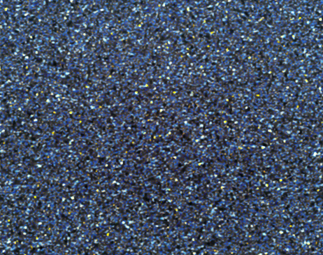
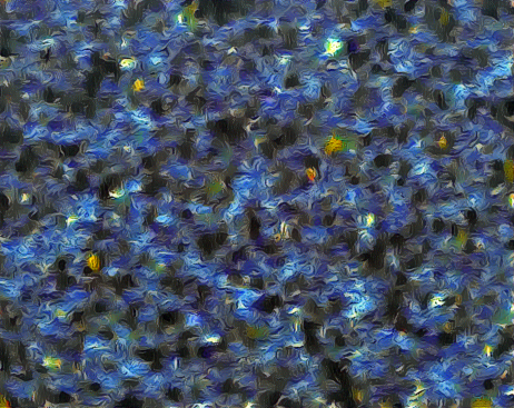
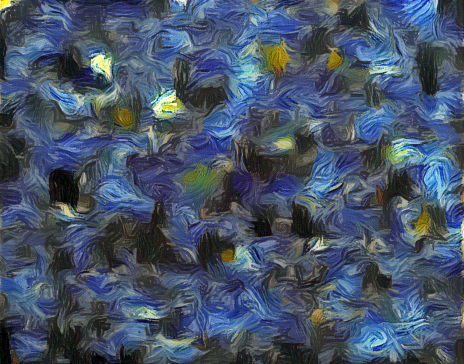
The graph below replicates a Figure 1 from the original paper. It shows two sets of reconstructed images: one generated by matching the content loss using feature maps from (a) conv1_1, (b) conv2_1, (c) conv3_1, (d) conv4_1, and (e) conv5_1; and another set obtained by applying only the style loss, using progressively larger subsets of layers: (a) conv1_1, (b) conv1_1, conv2_1, (c) conv1_1, conv2_1, conv3_1, (d) conv1_1, conv2_1, conv3_1, conv4_1, and (e) conv1_1, conv2_1, conv3_1, conv4_1, conv5_1.

Content reconstructions

Style representations

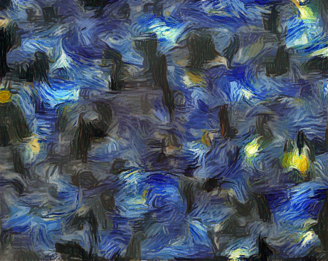
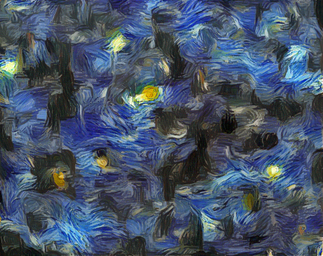
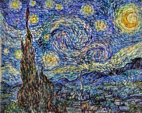
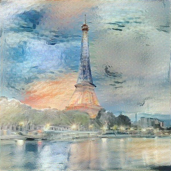
Since the most typical image used to extract the style is The Starry Night by Vincent van Gogh, I decided to apply the neural style transfer to a picture and another painting.

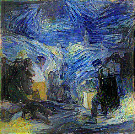
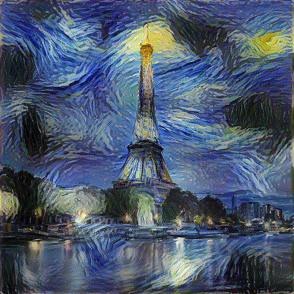
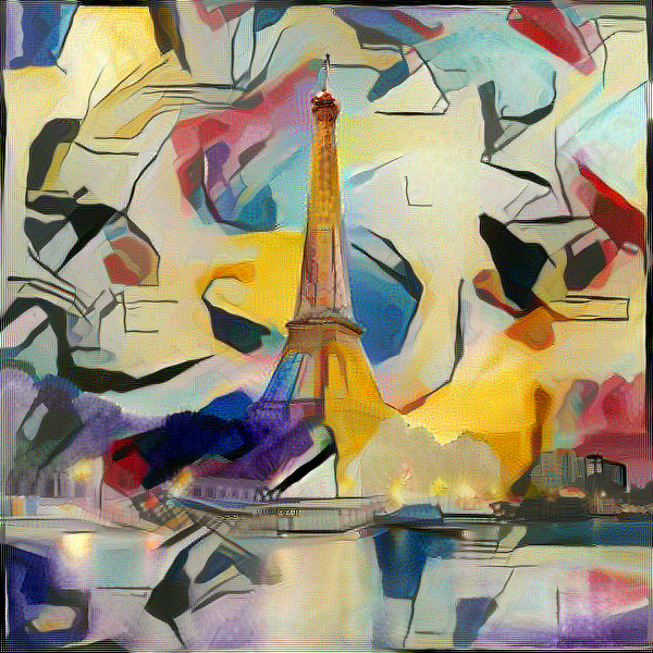
Finally I used the content of the Eiffel tower image apply some other styles. From what I experienced using paintings with very uniformly smooth defined styles such as The Starry Night or Impression, Soleil levant by Monet. However, when using more geometrical styles such as Gelb-Rot-Blau by Kandinsky or Guernica by Picasso the results were much less convincing.