Understanding Long Short-Term Memory

Recurrent Neural Networks (RNNs) are a type of neural network designed to process sequential data by retaining an internal memory of the previous inputs. This makes them particularly suited for problems such as speech recognition, non-Markovian control, or music composition.

However, in practice, training RNNs successfully was a challenge. Methods like Backpropagation Through Time (BPTT) or Real-Time Recurrent Learning (RTRL) suffer from vanishing or exploding gradients, making it difficult for RNNs to learn long-range dependencies.

This is the problem that Long Short-Term Memory (LSTM) networks were designed to solve when they were introduced in the Long Short-Term Memory seminal paper by Sepp Hochreiter and Jürgen Schmidhuber in 1997. LSTMs modified the recurrent architecture to create a constant error flow (Constant Error Carousel, or CEC) across time, allowing gradients to propagate over hundreds of steps without vanishing.

In this post, we’ll walk through the motivations, mathematical foundations, and original architectural decisions behind the LSTM formulation. We’ll start by examining why standard RNNs fail to retain long-term dependencies, explain the concept of error signals, and then follow the derivation that led them to the idea of the Constant Error Carousel (CEC), which is the key mechanism that allows LSTMs to overcome the vanishing gradient problem. From there, we’ll explore the full LSTM architecture, its advantages and limitations, how it has been used in practice, and its current relevance.

Exponentially Decaying Error in Conventional BPTT

First, they state that the contribution of the output error to the update of $w_{kl}$ is computed using by $\alpha \vartheta_k (t)y^l(t-1)$ with $\alpha$ the learning rate, $l$ an arbitrary unit connected to $k$ and $\vartheta_k$ the error signal at unit $k$ and time $t$, which is given by

for an output unit, for hidden units this error signal is given by

Yes, that’s a rough start. Let’s take one step back and understand where these formulas come from. First of all we have to understand the difference between error and error signal:

• Error is the difference between the output that our model predicts and the desired one. Normally, the sum of the square errors over the network output is taken as the error function. For instance, at time $t$ the error for unit $k$ is

where $d_k(t)$ is the desired output of unit $k$ at time $t$ and $y^k(t)$ is the output or activation of unit $k$ at time $t$.

• Error signal is a term that was borrowed from control theory and signal processing, but with a different definition. In the RNN context, it is defined as the partial derivative of the error function with respect to the total input (pre-activation) of unit $k$.

Error signal for output units

We can then expand the error signal using the chain rule:

where $net_k$ is the weighted sum of all incoming signals before applying the activation function

and $y^j(t)$ and $y^j(t-1)$ are the activations or output from time $t$ and the previous time step $t-1$ respectively. Note that the real implementation of the RNN would also include the external input $x(t)$, however the external input does not affect the error signal, so for clarity it is omitted in the paper. We can then compute each of the partial derivatives that make up the error signal after applying the chain rule. First by taking the partial derivative of the error function definition with respect to $y^k(t)$

and secondly by taking the partial derivative of $y^k(t)=f_k(net_k(t))$ with respect to $net_k(t)$

where $f'_k$ is the derivative of the activation function at unit $k$. By multiplying them we obtain the error signal for an output unit $k$:

Note that the minus sign is not included in the paper’s expression because it cancels out with the negative sign from gradient descent, which results in a positive term in the weight update rule.

Computing the output error signal was relatively easy as we have access to the desired outputs and the error function. But hidden units don’t have any of these, so how do we compute their error signals?

Error signal for hidden units

We can compute the error signal for hidden units by backpropagating the error from the units they feed into, this is called backpropagation through time (BPTT). The difficult part when computing the error signal for a hidden unit is the term $\frac{\partial E}{\partial y^k(t)}$ as there is no error function to be used, instead we have to use the errors from $t+1$ in order to backpropagate this term.

The output of all hidden units at time $t$ become part of the inputs to unit $k$ at $t+1$, such that

If we take the partial derivative of $net_k(t+1)$ with respect to a unit $j$ we just retain the jth element of the summation

We can then compute $\frac{\partial E}{\partial y^k(t)}$ applying the chain rule using the weighted input of the future state $net_i(t+1)$.

we are basically using the error signals of the next layer to obtain the current one. We can then compute each of the terms. First, by definition:

then the second term has already been computed before. By multiplying them we get

which allows us to derive the error signal for a hidden unit as

Note that the weight update equation which is normally defined as

where by using the chain rule again

since $net_j(t)=\sum_i w_{ji} y^i(t-1)$

so that finally the weight update equations is

note that the minus sign was taken into the output error signal.

Next, we analyze how the error signal from a unit $u$ at time $t$ propagates backward through time to affect a unit $v$ at time $t-q$. When there is only one timestep of difference we can directly compute the partial derivative of the hidden units error signal.

by unrolling the recursiveness the following general formulation can be obtained:

with $l_q=v$ and $l_0=u$. This formula is basically computing for all the possible paths that connect $u$ with $v$ the product of the weight connecting that path with the activation function derivative and summing them. Therefore there are a total of $n^{q-1}$ product terms, since the summation terms can have different sign increasing the number of units $n$ will not necessarily increase the error flow.

From that formula we can see that if $|f_{l_m}'\left( \text{net}_{l_m}(t - m) \right) w_{l_m l_{m-1}}|>1$ for all $m$, the product term will increase exponentially with $q$. Equally, if $|f_{l_m}'\left( \text{net}_{l_m}(t - m) \right) w_{l_m l_{m-1}}|<1$ then the product term decreases exponentially. In both cases, learning at the deeper layer will become impossible.

The vanishing local error flow problem can be extrapolated to the global error since this global error is the sum of the of the local error over the output units.

NAIVE CONSTANT ERROR FLOW

The error signal for a unit which is connected only to itself is given by

if we enforce a constant error flow through this unit ($\vartheta_k(t)=\vartheta_i(t+1)$)

we can then integrate this equation to obtain

which means that $f_k$ must be linear. In the original paper this is called Constant Error Carousel (CEC) and will be a key element in LSTM. Since the units of the CEC will not only be connected to themselves but also other units, a more complex approach is required to control the read and write operations in these units, as otherwise, conflicts may arise during weight updates. These interference and stability problems become worse as the time lag increases

LONG SHORT-TERM MEMORY

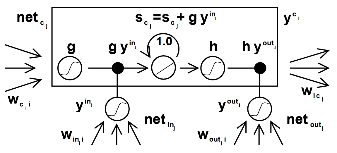
The naive Constant Error Carousel (CEC) enables constant error flow, but it lacks control over when information is written to or read from memory. To solve this, a multiplicative input gate was introduced to protect the memory contents of unit $k$ from being overwritten by irrelevant inputs. Similarly, a multiplicative output gate was added to prevent the memory content from affecting other units when it’s not needed. The resulting unit is called a memory cell, and it is built around the constant error carousel idea. The kth memory cell is referred to as $c_k$.

where

then, at time $t$, the output $y^{c_k}$ of $c_j$ is computed as

where the internal state is

The function $g$ squashes the input $net_{c_k}(t)$, producing a candidate value to be written into the memory cell. The function $h$ scales the output based on the internal state $s_{c_j}(t)$. We can distinguish two components in the update of $s_{c_j}(t)$. The first is the internal state from the previous timestep, $s_{c_j}(t-1)$. The second is the product $y^{in_k}(t) \cdot g(net_{c_k}(t))$, where $g(net_{c_k}(t))$ generates the data to write, and $y^{in_k}(t)$ decides whether this data should be written or ignored. Even though the output is passed through the non-linearity $h$, the Constant Error Carousel is still respected because the internal state $s_{c_j}(t)$ flows linearly through time within the memory cell.

Architecture

The networks used in the original paper consist of:

• One input layer, one hidden layer, and one output layer
• S memory cells sharing the same input gate and same output gate form a structure called memory cell block of size S.
• Real-Time Recurrent Learning (RTRL), a form of gradient descent, used for training .
• Update complexity that is linear in the number of weights $\mathcal{O}(W)$.

The authors noted that, during early training, the network may overuse the memory cells by keeping the gates open and exploiting the extra capacity. It is also possible for multiple cells to redundantly store the same information. To address these issues, they proposed:

• Sequential network construction by adding memory cells only when the error plateaus, rather than including them from the start
• Output gate bias: initialize each output gate with a negative bias to push initial activations toward zero and prevent premature memory usage

The paper includes a detailed description of six experiments of increasing complexity, where LSTM is benchmarked against traditional RNN training algorithms such as BPTT and RTRL. LSTM demonstrated a stronger capability to capture longer temporal dependencies.

From these experiments, the authors highlight the following advantages and limitations of LSTM:

Disadvantages

• LSTM cannot solve tasks like the strongly delayed XOR, because it uses truncated BPTT, which only allows error signals to propagate a fixed number of steps. Using full BPTT could help, but it’s computationally expensive.
• The need for input and output gates increases the number of parameters.
• For very long sequences (over 500 timesteps), LSTM tends to behave like a feedforward network that sees the entire input at once, and it suffers from similar limitations.
• LSTM lacks the ability to count exact numbers of timesteps between different events.

Advantages

• The use of the Constant Error Carousel (CEC) within memory cells allows LSTM to bridge long time lags. In the original implementation, the model was able to retain dependencies for up to 500 timesteps, a significant improvement over basic RNNs, which typically struggle beyond 20. For context, modern architectures such as Mamba can retain dependencies over millions of timesteps.
• LSTM requires little to no fine-tuning: it performs well across a wide range of learning rates, input gate biases, and output gate biases.
• LSTM is computationally efficient: the amount of computation per weight remains constant as the number of unrolled timesteps increases, it is $\mathcal{O}(1)$.

EVOLUTION, ACHIEVEMENTS AND PRESENT STATE

After the publication of this paper, considerable work was dedicated to further improve the LSTM architecture:

• In 2000, Gers et al. added a learnable forget gate, allowing a cell to reset its state when information became irrelevant ¹ , this is the current vanilla LSTM implementation nowadays.
• In 2000 Gers, Schmidhuber, and Cummins introduced peephole connections to allow each gate peek at the current cell value for finer timing control².
• Gated Recurrent Units (GRU) appeared in 2014, they merged gates and dropped the explicit cell state while matching LSTM accuracy with fewer parameters³.
• Finally, in 2024 Hochreiter introduced xLSTM⁴ (extendend LSTM) which allows to paralellize the training of LSTM in a similar fashion as with transformers.

LSTMs have been used in a wide variety of applications, ranging from speech and handwriting recognition to machine translation, time-series forecasting, and creative generation. Bidirectional LSTMs were employed in speech and online handwriting tasks, while Google’s first neural translation system used stacked LSTMs to significantly reduce error rates. They remain widely used in industrial forecasting and on-device anomaly detection, especially when long-range memory is needed but transformers are too resource-intensive.

However, since the rise of transformers in 2017, which scale better on modern hardware and achieve higher accuracy, LSTMs have declined in popularity. Furthermore, newer state-space models like Mamba can capture longer dependencies with fewer parameters.