Understanding Kalman Filters

In this post, I will talk about the probabilistic derivation of the Kalman filter, which is a nice introduction to a paper I intent to write in the near future, A Disentangled Recognition and Nonlinear Dynamics Model for Unsupervised Learning by M. Fraccaro et al. ¹

In short, the Kalman filtering deals with the task of finding the filtered posterior of a Linear Gaussian State Space Model, that is $p(\mathbf{z}_t\mid \mathbf{y}_{1:t}, \mathbf{u}_{1:t})$. There is also the Kalman smoother (or Rauch–Tung–Striebel smoother), which gives the smoothed posterior $p(\mathbf{z}_t\mid \mathbf{y}_{1:T}, \mathbf{u}_{1:T})$, note that the difference is that the smoother uses the entire sequence while the filter only uses data available up to the current time.

Many of the derivations in this post have been extracted from Probabilistic Machine Learning: Advanced Topics by Kevin Patrick Murphy ², which is a reference I cannot recommend enough to anyone interested in the topic.

Linear Gaussian State Space Model

State-space models (SSM) make use of the state variables to describe the system with a set of first-order differential (or differences) equations.

The SSM consist of:

• Hidden states $\mathbf{z}_t\in \mathbb{R}^{N_z}$ describe the system’s true internal condition, that evolves over time according to the dynamics or transition model.
• Inputs $\mathbf{u}_t\in \mathbb{R}^{N_u}$ are the external signals that influence the evolution of the hidden state.
• Observations $\mathbf{y}_t \in \mathbb{R}^{N_y}$ are the measured quantities of the system.
• Process noise $\mathbf{q}_t$ is the uncertainty of how the hidden state evolves over time. This can be due to random disturbances and modeling simplifications among others.
• Observation noise $\mathbf{r}_t$ is the uncertainty in the sensor measurements.

For instance: for a rocket, the hidden state could be the position and velocity, the input would be the amount of thrust delivered by the engines and the observation could consist of the altitude measurements. The process noise could come from unexpected winds, or differences in the expected atmospheric density. The observation noise could be random biases of the sensor, drifts, etc.

The SSM is normally written as a probabilistic model given by the dynamics model or transition model $p(\mathbf{z}_t \mid \mathbf{z}_{t-1}, \mathbf{u}_t)$ and observation model or measurement model $p(\mathbf{y}_t \mid \mathbf{z}_t, \mathbf{u}_t, \mathbf{y}_{1:t-1})$.

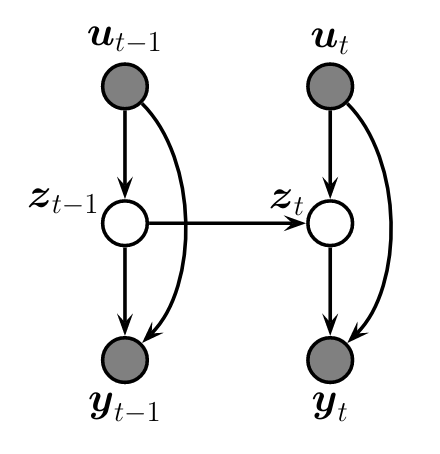
The figure below shows the graphical model of the state-space model

If $\mathbf{f}$ and $\mathbf{h}$ are linear functions then we have a linear-Gaussian SSM (LGSSM), this is normally written as

where $\mathbf{A}_t$ is the state transition matrix, $\mathbf{B}_t$ the control-input matrix, $\mathbf{C}_t$ the observation matrix, and $\mathbf{D}_t$ the feed-through matrix, which maps the input $u_t$ directly to the observation and is often 0 as normally inputs affect the observations only through the state.

Also, normally we assume that the process and observation noises are multivariable Gaussian-distributed random variables with mean 0 and some covariance.

There are two strong reasons for modelling this noises as Gaussian.

• They are stable by linear transformation, which means that we can easily propagate uncertainty.
• They are stable by conditioning. Which means that if we have a Gaussian likelihood and prior the posterior will also be Gaussian.

Since any linear transformation of a multivariate normal distribution is also multivariate normally distributed we can rewrite the transitions and observation model as

Note that we assume the standard Markov observation model in which $\mathbf{y}_t \bot \mathbf{y}_{1:t-1}\mid (\mathbf{z}_t, \mathbf{u}_t)$, that is the current observation is independent of the previous observations given the current latent state and control.

Likelihood, Posterior and Prior Beliefs

The goal of the Kalman filter is then to compute the posterior distribution of the hidden state given all measurements and controls so far:

by direct application of the Bayes rule (Posterior = Likelihood × Prior / Evidence)

to the posterior distribution we obtain

note that $u_{1:t}$ are known so they are always given and not random variables. We can then use the chain rule in the numerator, and use the property that in the SSM the current observation only depends on the current state and current input

The denominator can be expressed as the marginalized joint distribution, then substitute the expression above and take outside of the integral the terms that do not depend on $\mathbf{z}_{t}$

we write numerator and denominator as

In the Bayesian paradigm, the concepts of posterior, likelihood and prior are extremely important.

First, the likelihood relates the data with a set of parameters. In the Kalman filter this relates the observations $\mathbf{y}_t$ with the current state $\mathbf{z}_t$ and control $\mathbf{u}_t$. This likelihood is directly obtained from the observation model defined above.

It reads as the probability of getting a measurement $\mathbf{y}_t$ for a given state $\mathbf{z}_t$ and control $\mathbf{u}_t$.

The prior is our belief of the state before seeing a measurement.

Since both the likelihood and the prior are multivariate Gaussians the result will be a Gaussian as well, since the evidence is a constant that scales the resulting distribution, in practice it is dropped, as we only care about the mean and covariance of the posterior to compute the Kalman filter.

The Kalman Filter

The Kalman Filter is the algorithm to obtain the exact Bayesian filtering for Linear Gaussian State Space Models, it finds $p(\mathbf{z}_t \mid \mathbf{y}_{1:t}) = \mathcal{N}(z_t| \mathbf{\mu}_{t|t}, \mathbf{\Sigma}_{t|t})$ where $\mathbf{\mu}_{t|t}, \mathbf{\Sigma}_{t|t}$ refer to the posterior mean and covariance given the observations $\mathbf{y}_{1:t}$ and the control $\mathbf{u}_{1:t}$. Note that there is an analytically close form because all the distributions are Gaussian.

The algorithm consist in a predictor, which get the one-step prediction using the transition model,

Predictor step

The predictor step involves the computation of the prior. First of all note that if $\mathbf{z}_{t-1}$ were known, the distribution of $\mathbf{z}_{t}$ would simply be

however, $\mathbf{z}_{t-1}$ is the hidden state so we only know its distribution

using the total law of probability and the fact that $\mathbf{z}_{t}$ is independent of $\mathbf{y}_{1:t-1}$ given $\mathbf{z}_{t-1}$ we integrate over the uncertainty in $\mathbf{z}_{t-1}$

the second term in the integral is Gaussian and the first term of the integral is the transition model, which is also Gaussian

we can express the product then as the joint Gaussian over the stacked vector

Then the mean of the joint is

and then compute the covariances

to assemble the matrix

Finally note that to marginalize in a joint distribution one simply drops the irrelevant variables (the ones to marginalize) from the mean vector and covariance matrix, in our case we marginalizing with respect to $\mathbf{z}_{t-1}$ we remain with

Note that if no new measurements are used in the update step then the covariance grows with time.

Corrector (Update) step

The corrector step compute the posterior by using the likelihood (measurement model) and the prior from the predict step.

In order to solve this we will build the joint distribution $p(\mathbf{z}_t,\mathbf{y}_t \mid \mathbf{y}_{1:t-1}, \mathbf{u}_{1:t})$ and then take the conditional distribution inside the joint Gaussian $p(\mathbf{z}_t\mid \mathbf{y}_t, \mathbf{y}_{1:t-1}, \mathbf{u}_{1:t})$. First, we define the joint Gaussian

and compute the joint mean

and each joint covariance

so that the covariance matrix is

where $\mathbf{S}_t = \mathbf{C}_t\,\boldsymbol{\Sigma}_{t|t-1}\,\mathbf{C}_t^{T}+\mathbf{R}_t$ is called the innovation covariance. Then the conditional distribution of a general joint Gaussian is ³

We start by substituting terms in the mean to get the mean of the posterior

where $\mathbf{K}_t$ is called the Kalman gain matrix

then, we proceed in the same way but with the covariance

so that we have the mean and covariance of the posterior