Introduction to Convolutional Neural Networks

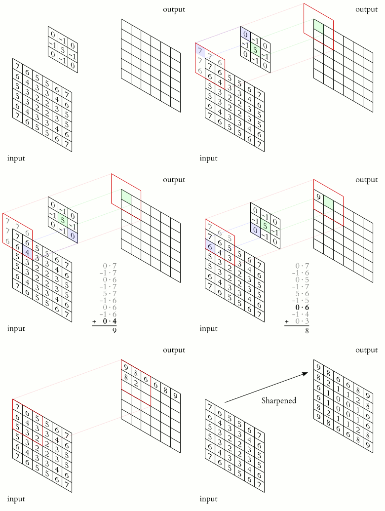
Convolutional neural networks were popularized in 1998 by LeCun, Bottou et al. ¹ when they introduced LeNet-5 for digit recognition, which was later applied to the recognition of ZIP code digits by the U.S. Postal Service. The main idea in convolutional neural networks (CNNs) is that, rather than connecting all the units (neurons) in one layer to all the units in the next one —as is the case in an Multilayer perceptron MLP—convolutional networks consist in sliding filters —also called kernels— over the original image or input, forming the so-called feature map. Several feature maps are then stacked creating the output of that layer.

One of the main reasons for using CNNs is that they are very efficient for processing images where there is a known data structure because the paramters —or weights— of the filters in each layer are the same for all pixels in the input, so there are overall fewer weights to learn compared to a fully connected network. They are also very useful to exploit the spatial invariance of images, by creating local feature layers which are successively combined to create more meaningful and complex features.

Convolutional Layer

Let $\boldsymbol{X}$ be a matrix with the input image, and $\boldsymbol{H}$ be the successive hidden layer. Then we can write the convolutional operation that takes us from $\boldsymbol{X}$ to $\boldsymbol{H}$ as

where $b$ is the bias term, $\boldsymbol{W}$ defines the filter, also called the weight matrix or convolution kernel, and $2\Delta+1$ is the size of the kernel (assumed squared here).

So far we assumed that the input image is given by just a matrix, however, real images consist of three channels red, green, and blue (RGB), so they are third-order tensors rather than matrices. These tensors are characterized by their height, width, and channel. In the CNN jargon height and width are the spatial coordinates while the channels are referred to as the depth. As an example, a 1920x1080 image will be represented by a 1920x1080x3 tensor.

The concept of convolutional neural network is closely related to that of image convolution and the mathematical concept of convolution, however, there are some key differences that are worth pointing out:

• While image convolutions apply normally the same filter to each color channel of the image, in CNNs the approach is different, all channels from the previous layers are linearly combined using a filter with the same depth —number of channels. Extending the formulation already used, the tensor representation of the convolutional operation would be as the formular below where $c$ is the input channels (three for the first layer). In practice, every layer is formed by several filters $d$, and the output of these filters is then stacked to form a hidden layer with depth $d$.

• Mathematical convolution is defined as $(f * g)(x) = \int f(z)g(x-z)dz$ where the function $g$ is flipped and shifts to perform the convolution operation. In CNNs, the kernels are not flipped, so in formal terms, the operation would be a cross-correlation and not a convolution, however, this term is used loosely in the CNN field. For more insight into the mathematical convolution, I strongly recommend the video What is a convolution? from 3Blue1Brown.

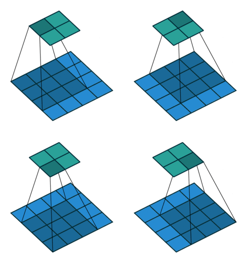
Up to this point, we’ve seen that each convolution layer will be defined by the spatial size of the filters and also the number of filters, which will define the depth of the output layer. Additionally, other parameters that will define the convolutional layer and allow for more control over the size of the output include padding, stride, dilation, and grouping.

Padding

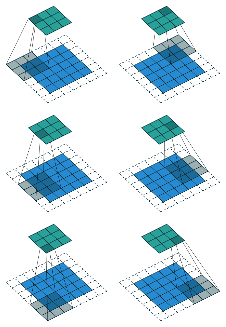
Padding is used to avoid convolutions reducing largely the size of the output. As a matter of fact, convolving a kernel of size $k$ over an input image of shape $n\times n$ will give an output size:

because we can only shift the convolutional kernel until it runs out of pixel to apply the convolution. The first CNNs such as LeNet-5 did not use padding, which meant the size shrank on each convolution layer.
In order to solve this problem, extra pixels can be added around the frame of the input image to increase its size. Normally, the value of the padding is set to zero, although pixel replication methods such as wrap, clamp, or mirroring can also be used. Alsallakh et al. (2020)² presented an extensive overview of the existing alternatives to zero-padding.

From Szeliski.

When using padding $p$ (number of rows/columns surrounding the input image), the size of the output layer is

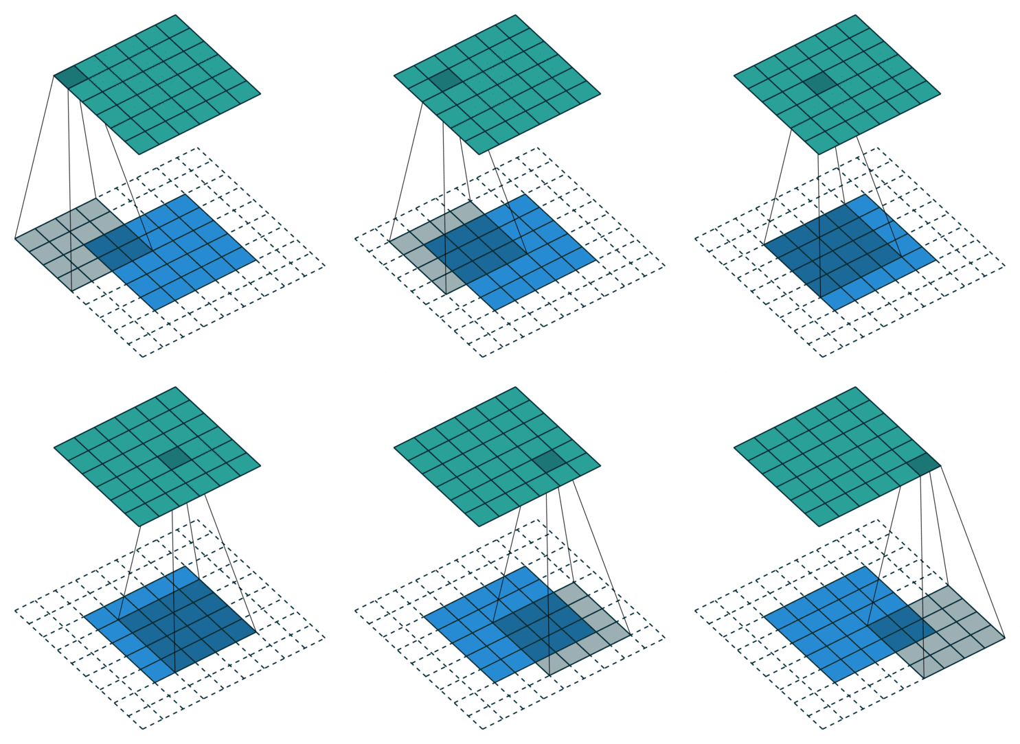
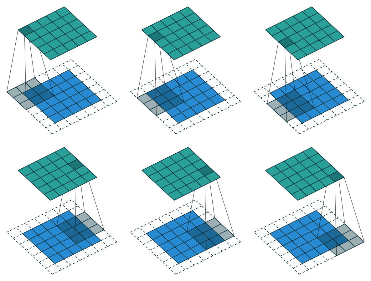
Note that when using a padding $p=\frac{k-1}{2}$ the input and output will have the same size if $k$ is even. Otherwise, there will be a difference between the top/left and bottom/right padding which will be computed as $\lceil \frac{k-1}{2} \rceil$ and $\lfloor \frac{k-1}{2} \rfloor$. For this reason, normally convolution kernels have odd sizes so that the padding remains symmetric with the same number of top/bottom rows and left/right columns.

Stride

It refers to the amount of pixels the filter is slid when computing the cross-correlation. By default this value is normally 1, however, for reasons such as computational efficiency or to downsample the input, we can slide by skipping intermediate pixels. For instance, the stride for the first layer in AlexNet had a stride of 4, and traditional image pyramids use a stride of 2 in the coarser levels. The output dimension of a convolution operation with stride $s$ is

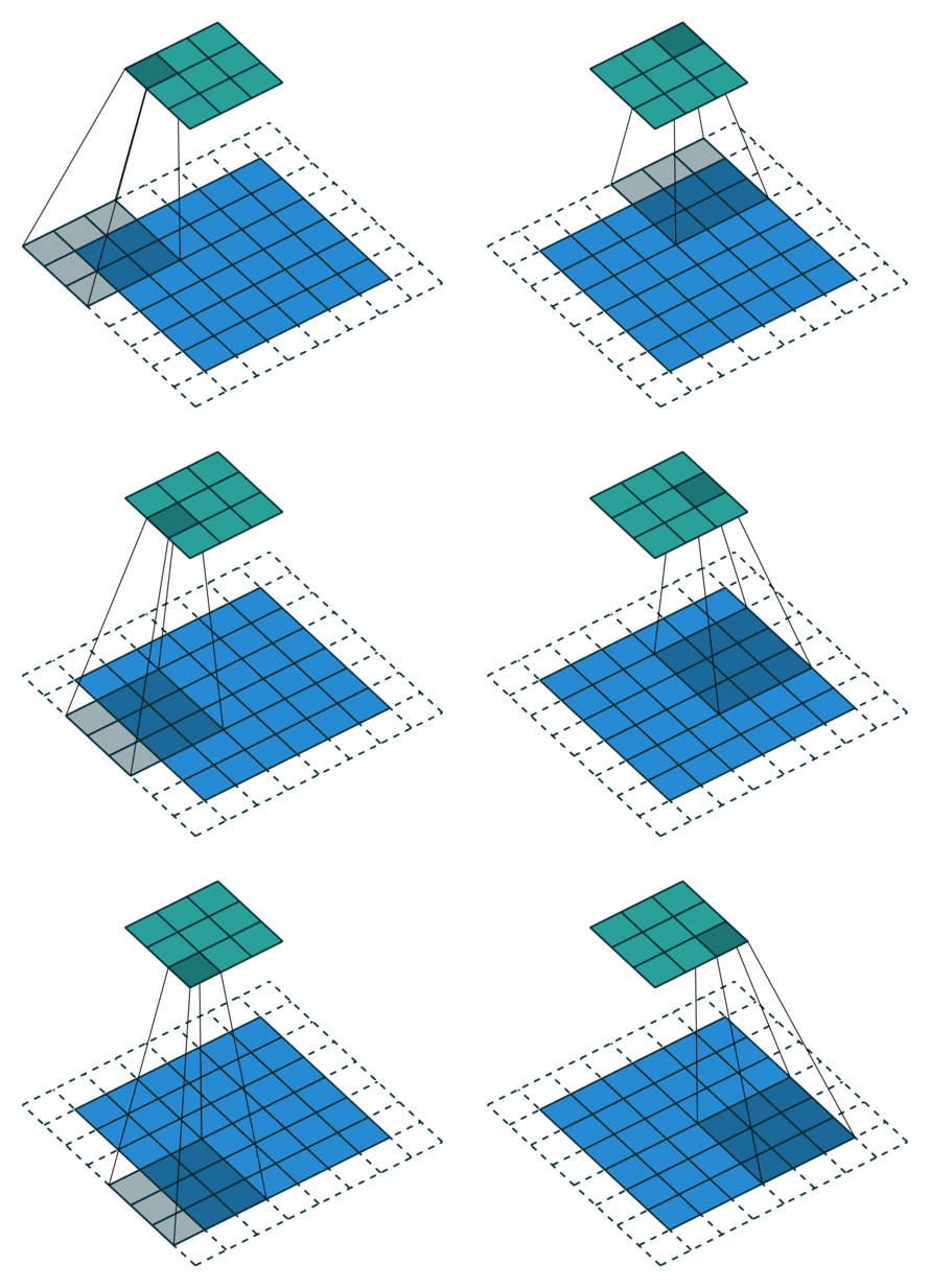
In general, when the input image, filter, padding, and strides are not squares, the output shape will be given by

Dilation

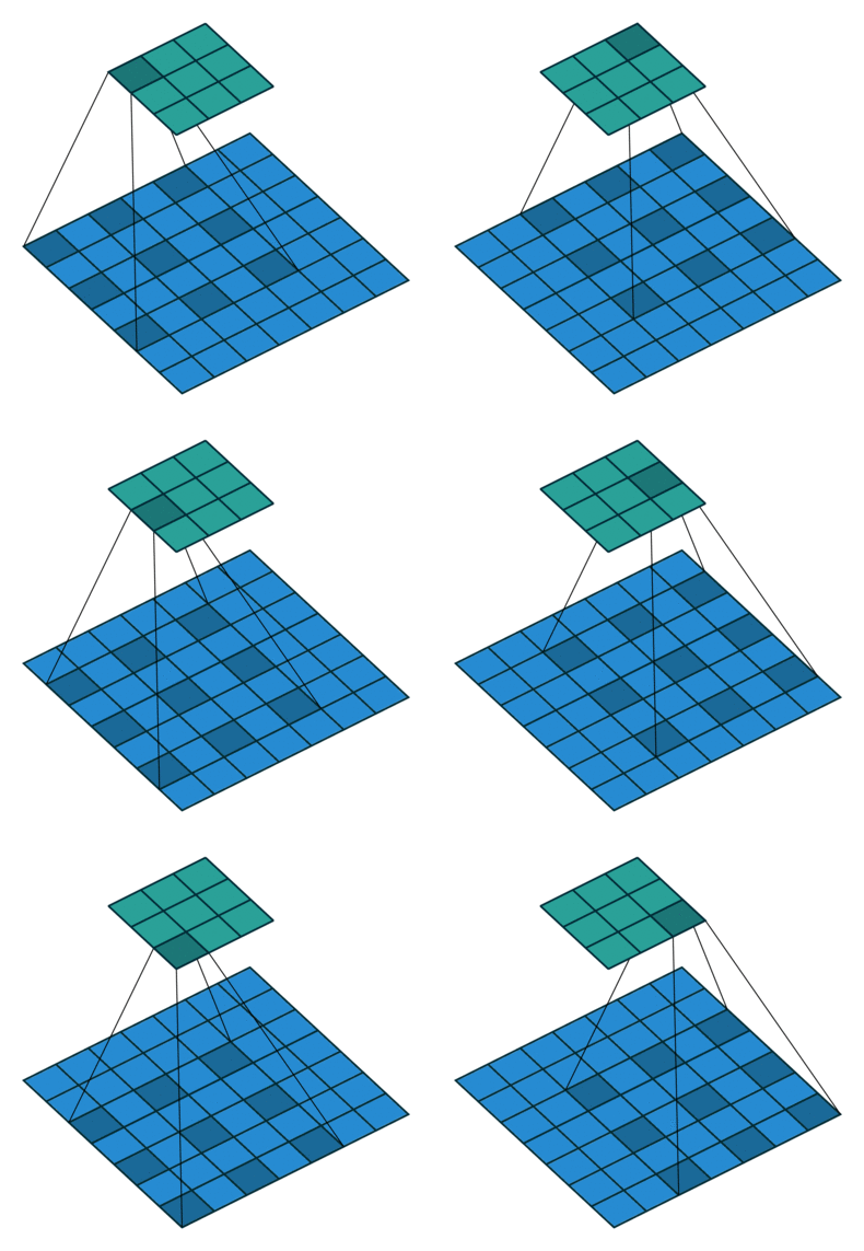
We call dilation when extra space is inserted between the pixels sampled during the convolution, this is also called atrous (from French a trous). ^{3 4}

Grouping

It’s used when we group the input and output layers into separate groups which are convoluted separately. If $G=1$ then it is the regular convolution (using all channels) otherwise each channel is convolved independently from the other, this is also known as depthwise or channel-separated convolution. ^{5 6 7}

Output dimension calculator

Click on the following link for a interactive calculator of the output layer shape, based on all the variables we have learnt so far.

Pooling

The pooling operator consist, like with convolution layers, of a window that slides over the input and computes a single output at each location. However, there are two key differences between pooling and cross-correlation layers:

• Pooling layers have no parameters to learn (no kernel), so the operator is fixed beforehand. The typical pooling operators consist of computing the average value (average pooling or even L2-norm pooling) and computing the maximum value (max-pooling), introduced in 1999 by Riesenhuber and Poggio⁸ in the context of cognitive neuroscience.

• While cross-correlation layers are applied to all input channels, pooling is typically applied to each channel independently.

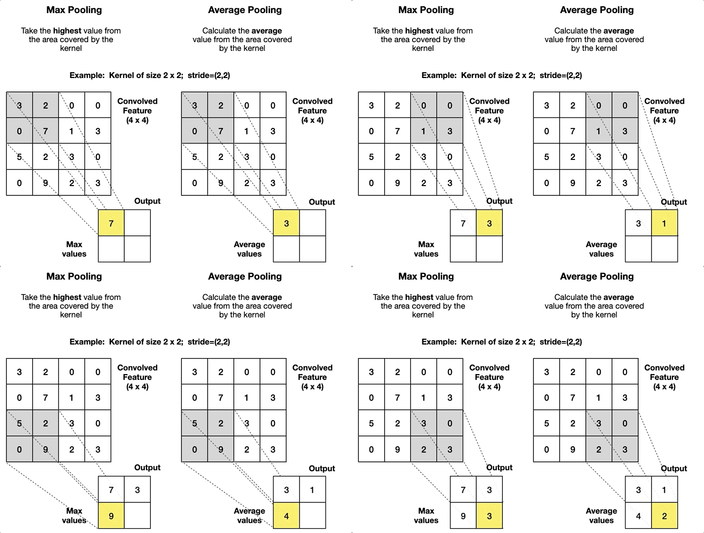
Pooling layers are added to the convolutional architecture to mitigate the sensitivity of the CNN to translation and to downsample the representations. The idea behind pooling is that features can shift relative to each other so that a robust matching of features can be done even when small distortions occur while also reducing the spatial dimension of the feature map. This operator is also used in other methods like in the scale-invariant feature transform (SIFT) descriptor with a 4×4 sum pooling grid.

In general, pooling layers use a value of stride equal to the size of the pooling window since the pooling operator aggregates information from an area. In practice max-pooling is preferable to average pooling in almost all cases, and the two most popular variations of max-pooling are:

• Size 2 & stride 2
• Size 2 & stride 3 (called overlapping pooling)

since larger sizes or larger strides are too destructive

Pooling layers are a bit outdated and nowadays many people are proposing to discard them and prioritize architectures using just repeated convolutional layers.⁹ The idea is to use layers with large strides once in a while to reduce the size of the feature map. Discarding pooling layers was found to be important in training good generative models, such as variational autoencoders (VAEs) and generative adversarial networks (GANs), and seems to be the trend for the future.