Implementing VGGNet from Scratch Using PyTorch
Posted on 2/21/2025
In this post, I will implement and train VGGNet using PyTorch, building on my previous AlexNet implementation. The post will be structured as follows: first, we will create the network architecture, followed by data processing, speed optimizations, the training loop, training results, and conclusions. By the end, we will have a clear idea of how to implement VGGNet using PyTorch and how its performance compares to the original paper.
VGGNet Architecture
The goal of this implementation is to create a generic class that can be used to define and train any of the VGGNet configurations, excluding those that use LRN and 1×1 convolutions. Unlike AlexNet, where layers were manually coded, this implementation must be done programmatically. However, the consistent and systematic architecture of VGGNet will simplify the process.
As you might recall from my previous post, every VGGNet configuration consists of:
- Convolutional blocks, each containing a variable number of convolutional layers with a constant number of channels, followed by a max pooling layer.
- Two classifier blocks:
- A fully connected classifier for training.
- A convolutional and sum-pooling classifier for performing dense evaluation during testing.
Each convolutional block will be created using the create_conv_block function. This function generates num_convs convolutional layers using 3×3 kernels and the ReLU activation function. Note that each convolutional layer uses the same number of filter channels, which is ensured by setting in_channels = out_channels within the loop. Each convolutional block is followed by a max-pooling layer with a kernel size of 2 and a stride of 2. At the end, all layers are passed to nn.Sequential, which constructs the convolutional block.
    def create_conv_block(in_channels, out_channels, num_convs):
        layers = []
        for _ in range(num_convs):
            layers.append(nn.Conv2d(in_channels, out_channels, kernel_size=3, stride=1, padding=1))
            layers.append(nn.ReLU(inplace=True))
            in_channels = out_channels

        layers.append(nn.MaxPool2d(kernel_size=2, stride=2))
        return nn.Sequential(*layers)
Since the number of filter channels for each block follows the simple rule of doubling every layer up to 512, namely [64, 128, 256, 512, 512], each VGGNet configuration will be uniquely defined by a list indicating the number of convolutional layers within each block. For example, VGG11 is represented as [1, 1, 2, 2, 2], and VGG16 as [2, 2, 3, 3, 3]. Hence, the first convolutional block of any VGGNet model will be created as:
create_conv_block(in_channels=3, out_channels=64, num_convs=conv_config[0])The classifier is common to all configurations and consists of 3 layers and it’s also created using nn.Sequential. Bear in mind that, when using 227×227 input images and computing the output size after passing through all convolutional blocks (using the ConvNet calculator), we find that the final output has a shape of 7×7×512. This determines the input size of the first linear layer.
# Fully connected classifier for training
classifier = nn.Sequential(
	nn.Linear(512 * 7 * 7, 4096),
	nn.ReLU(inplace=True),
	nn.Dropout(p=0.5),
	nn.Linear(4096, 4096),
	nn.ReLU(inplace=True),
	nn.Dropout(p=0.5),
	nn.Linear(4096, num_classes)
)
The convolutional classifier is used to perform dense evaluation during testing and allows processing images of variable sizes rather than being limited to 227×227 RGB images. Due to how the kernels of this classifiers are designed, if the input is larger, the output of the convolutional classifier will no longer be a vector but rather a tensor of shape (>1)×(>1)×1000. In order to transform this tensor into a vector, the original paper uses sum-pooling. Instead of sum-pooling, I used adaptive average pooling, as it is the only adaptive method directly available in PyTorch.
# Convolutional classifier for dense evaluation
conv_classifier = nn.Sequential(
	nn.Conv2d(512, 4096, kernel_size=7),
	nn.ReLU(inplace=True),
	nn.Conv2d(4096, 4096, kernel_size=1),
	nn.ReLU(inplace=True),
	nn.Conv2d(4096, num_classes, kernel_size=1),
	nn.AdaptiveAvgPool2d(1)
)
The parameters were initialized using Xavier initialization with nn.init.xavier_uniform_. This avoids the need to first train VGG11 and then transfer its weights to a larger model to use the pretrained parameters as an initial guess for the optimizer.
Another method was created to transform and transfer the weights from the fully connected classifier to the convolutional classifier. This method is called at the beginning of the test loop.
The separation between the fully connected classifier and the convolutional classifier during the forward pass is determined by evaluating self.training, an attribute of nn.Module that indicates whether the model is in training or inference (evaluation) mode.
The code below includes the complete PyTorch implementation of a generic VGGNet, which can be configured to use 11, 13, 16, or 19 layers, depending on the configuration we want to use.
class VggNet(torch.nn.Module):
    def __init__(self, num_classes=1000, vgg=16):
        """
        VGGNet implementation for image classification.

        Args:
            num_classes (int, optional): Number of output classes. Default is 1000 (for ImageNet).
            vgg (int, optional): VGG configuration, either 11, 13, 16 or 19 for VGG-11, VGG-16 or VGG-19.
                                    Default is 16.
        """
        super(VggNet, self).__init__()
        self.num_classes = num_classes

        if vgg not in (11, 13, 16, 19):
            raise ValueError("vgg must be 11, 13, 16, or 19")

        # Configurations:
        # VGG-11: [1, 1, 2, 2, 2]
        # VGG-13: [2, 2, 2, 2, 2]
        # VGG-16: [2, 2, 3, 3, 3]
        # VGG-19: [2, 2, 4, 4, 4]
        if vgg == 11:
            conv_counts = [1, 1, 2, 2, 2]
        elif vgg == 13:
            conv_counts = [2, 2, 2, 2, 2]
        elif vgg == 16:
            conv_counts = [2, 2, 3, 3, 3]
        else:  # vgg == 19
            conv_counts = [2, 2, 4, 4, 4]

        # Build convolutional blocks
        self.block1 = self._create_conv_block(in_channels=3,   out_channels=64,  num_convs=conv_counts[0])
        self.block2 = self._create_conv_block(in_channels=64,  out_channels=128, num_convs=conv_counts[1])
        self.block3 = self._create_conv_block(in_channels=128, out_channels=256, num_convs=conv_counts[2])
        self.block4 = self._create_conv_block(in_channels=256, out_channels=512, num_convs=conv_counts[3])
        self.block5 = self._create_conv_block(in_channels=512, out_channels=512, num_convs=conv_counts[4])

        # Fully connected classifier for training mode (after flattening)
        self.classifier = nn.Sequential(
            nn.Linear(512 * 7 * 7, 4096),  # for 224x224 input images
            nn.ReLU(inplace=True),
            nn.Dropout(p=0.5),
            nn.Linear(4096, 4096),
            nn.ReLU(inplace=True),
            nn.Dropout(p=0.5),
            nn.Linear(4096, num_classes)
        )

        # Save fully connected layers to transfer weights later on
        self.fc1 = self.classifier[0]
        self.fc2 = self.classifier[3]
        self.fc3 = self.classifier[6]

        # Convolutional classifier for evaluation
        self.conv_classifier = nn.Sequential(
            nn.Conv2d(512, 4096, kernel_size=7),
            nn.ReLU(inplace=True),
            nn.Conv2d(4096, 4096, kernel_size=1),
            nn.ReLU(inplace=True),
            nn.Conv2d(4096, num_classes, kernel_size=1),
            nn.AdaptiveAvgPool2d(1)
        )

        # Weight initialization recursively to all submodules
        self.apply(self._initialize_weights)

    def _create_conv_block(self, in_channels, out_channels, num_convs):
        """
        Create a convolutional block as:
        [num_convs x (Conv2d -> ReLU)] -> MaxPool2d

        Args:
            in_channels (int): Number of input channels.
            out_channels (int): Number of output channels.
            num_convs (int): Number of convolutional layers in the block.
        Returns:
            nn.Sequential: The convolutional block.
        """
        layers = []
        for _ in range(num_convs):
            layers.append(nn.Conv2d(in_channels, out_channels, kernel_size=3, stride=1, padding=1))
            layers.append(nn.ReLU(inplace=True))
            in_channels = out_channels  # the next convolution uses out_channels as input

        layers.append(nn.MaxPool2d(kernel_size=2, stride=2))
        return nn.Sequential(*layers)

    def _initialize_weights(self, module):
        """
        Initialize the weights using Xavier uniform initialization.
        """
        if isinstance(module, (nn.Conv2d, nn.Linear)):
            nn.init.xavier_uniform_(module.weight)
            if module.bias is not None:
                nn.init.constant_(module.bias, 0.0)

    def fc2conv_weights(self):
        """
        Convert the fully connected classifier weights to convolutional weights for dense evaluation.
        """
        with torch.no_grad():
            # First FC layer to first conv layer
            self.conv_classifier[0].weight.copy_(self.fc1.weight.view(4096, 512, 7, 7))
            self.conv_classifier[0].bias.copy_(self.fc1.bias)

            # Second FC layer to third conv layer
        self.conv_classifier[2].weight.copy_(self.fc2.weight.view(4096, 4096, 1, 1))
            self.conv_classifier[2].bias.copy_(self.fc2.bias)

            # Third FC layer to fifth conv layer
self.conv_classifier[4].weight.copy_(self.fc3.weight.view(self.fc3.out_features, 4096, 1, 1))
            self.conv_classifier[4].bias.copy_(self.fc3.bias)

    def forward(self, x):
        x = self.block1(x)
        x = self.block2(x)
        x = self.block3(x)
        x = self.block4(x)
        x = self.block5(x)

        if self.training:
            x = torch.flatten(x, 1)
            x = self.classifier(x)
        else:
            x = self.conv_classifier(x)
            # Reshape (n_batch, n_classes, 1, 1) to (n_batch, n_classes)
            x = x.squeeze(-1).squeeze(-1)

        return x
We can use torchsummary to obtain a summary of each model. The output below shows the summary for VGG16. We can see that while there are 138,357,544 unique parameters, the model contains 262,000,400 parameters in total due to the duplication of the linear and convolutional classifiers, which is indeed suboptimal and could be improved. This also explains why the model parameters weigh around 1GB. Additionally, we can see that the classifier accounts for approximately 90 percent of the model’s total weight, highlighting the efficiency of CNNs.
----------------------------------------------------------------
        Layer (type)               Output Shape         Param #
================================================================
            Conv2d-1        [256, 64, 227, 227]           1,792
              ReLU-2        [256, 64, 227, 227]               0
            Conv2d-3        [256, 64, 227, 227]          36,928
              ReLU-4        [256, 64, 227, 227]               0
         MaxPool2d-5        [256, 64, 113, 113]               0
            Conv2d-6       [256, 128, 113, 113]          73,856
              ReLU-7       [256, 128, 113, 113]               0
            Conv2d-8       [256, 128, 113, 113]         147,584
              ReLU-9       [256, 128, 113, 113]               0
        MaxPool2d-10         [256, 128, 56, 56]               0
           Conv2d-11         [256, 256, 56, 56]         295,168
             ReLU-12         [256, 256, 56, 56]               0
           Conv2d-13         [256, 256, 56, 56]         590,080
             ReLU-14         [256, 256, 56, 56]               0
           Conv2d-15         [256, 256, 56, 56]         590,080
             ReLU-16         [256, 256, 56, 56]               0
        MaxPool2d-17         [256, 256, 28, 28]               0
           Conv2d-18         [256, 512, 28, 28]       1,180,160
             ReLU-19         [256, 512, 28, 28]               0
           Conv2d-20         [256, 512, 28, 28]       2,359,808
             ReLU-21         [256, 512, 28, 28]               0
           Conv2d-22         [256, 512, 28, 28]       2,359,808
             ReLU-23         [256, 512, 28, 28]               0
        MaxPool2d-24         [256, 512, 14, 14]               0
           Conv2d-25         [256, 512, 14, 14]       2,359,808
             ReLU-26         [256, 512, 14, 14]               0
           Conv2d-27         [256, 512, 14, 14]       2,359,808
             ReLU-28         [256, 512, 14, 14]               0
           Conv2d-29         [256, 512, 14, 14]       2,359,808
             ReLU-30         [256, 512, 14, 14]               0
        MaxPool2d-31           [256, 512, 7, 7]               0
           Linear-32                [256, 4096]     102,764,544
           Linear-33                [256, 4096]     102,764,544
             ReLU-34                [256, 4096]               0
          Dropout-35                [256, 4096]               0
           Linear-36                [256, 4096]      16,781,312
           Linear-37                [256, 4096]      16,781,312
             ReLU-38                [256, 4096]               0
          Dropout-39                [256, 4096]               0
           Linear-40                [256, 1000]       4,097,000
           Linear-41                [256, 1000]       4,097,000
================================================================
Total params: 262,000,400
Trainable params: 262,000,400
Non-trainable params: 0
----------------------------------------------------------------
Input size (MB): 150.96
Forward/backward pass size (MB): 56906.53
Params size (MB): 999.45
Estimated Total Size (MB): 58056.95
----------------------------------------------------------------
Data Processing
The preprocessing applied to ImageNet is exactly the same as the one used for AlexNet, so I refer to the Implementing AlexNet post for details on that. The data processing during training time for augmentation includes all the methods explained in the previous post, plus scale jitter.
- Scale Jitter: I used PyTorch’s Resize method within a lambda to apply a random scale jitter within the interval [256, 512].
def scaleJitter(x, min_size=256, max_size=512):
    S = random.randint(min_size, max_size)
    return transforms.Resize(S, antialias=True)(x)
During testing, the original paper proposes three alternatives: use dense evaluation (multi-scale, where the images are evaluated at different scales, namely 256, 384, and 512), use multi-crop (with 50 crops per image instead of the FiveCrop used in AlexNet), or use both methods (which implies 150 evaluations per image). Since using multi-crop as described in the paper would increase the number of evaluations per image by a factor of 50, and even the authors discourage using it due to the increased computation load compared to the gains in accuracy, I decided to just use dense evaluation. Additionally, using dense evaluation to transform the fully connected classifier into a convolutional to allow evaluating images of different sizes was something new compared to the implementation of AlexNet. The code below implements the transformation used for testing.
def multiResize(x):
    resized_images = [transforms.Resize(size, antialias=True)(x) for size in [256, 384, 512]]
    return resized_images
Finally, all these individual transformations were combined using transforms.Compose. Two different transformations were created: one for training, which includes random transformations for data augmentation, and one for testing, which includes the multi-scale transformation and removes random transformations to ensure determinism.
transform_train = transforms.Compose([
    # Apply PCA color transformation
    transforms.Lambda(PCAColorAugmentation),
    # Remove mean
    transforms.Lambda(meanSubstraction),
    # Scale jitter between 256 and 512
    transforms.Lambda(scaleJitter),
    # 224x224 random crop
    transforms.RandomCrop(224),
    # Horizontal reflection with p=0.5
    transforms.RandomHorizontalFlip(p=0.5),
])

transform_val = transforms.Compose([
    # Transform to tensor without scaling
    transforms.Lambda(toTensorNoScaling),
    # Remove mean
    transforms.Lambda(meanSubstraction),
    # Resize to 256, 384 and 512
    transforms.Lambda(multiResize),
])
Speeding up training
Since these VGGNets are very deep convolutional networks, optimizing the runtime of one epoch will be critical. This time, I will be using all the methods that were discarded in the AlexNet implementation, along with some new ones, as I will not be running the training on my personal laptop, but on a paid service on the cloud.
- CPU to GPU: Using the GPU instead of the CPU for training is, obviously, the first improvement. We can move a model or variable to the GPU using
.to(device), wheredeviceis set to the GPU if available, otherwise, it will default to the CPU. To ensure compatibility across different machines, we can definedeviceas follows:
device = torch.device('cuda' if torch.cuda.is_available() else 'cpu')- Model Compilation: PyTorch provides an easy way to compile models for faster training. Compiling a model is as simple as running
torch.compile(model). - Automatic Mixed Precision (AMP): PyTorch includes a mechanism to automatically switch from FP32 (full-precision floating-point format) to FP16 (half-precision floating-point format), allowing certain operations to run faster without significant loss of accuracy.
The first step to perform AMP is to initialize the gradient scaler torch.cuda.amp.GradScaler outside of the epoch training function. Gradient scaling is applied to ensure that very small gradient values, which may not be representable with float16 and could become zero, do not produce underflow. By scaling the gradients, they become larger and are not transformed to zero.
scaler = torch.cuda.amp.GradScaler()The next step is to allow regions of the script to run in mixed precision by invoking torch.cuda.amp.autocast(). Normally, we only wrap the forward pass and loss computation, while the backward pass is kept outside using the scaler. Overall, this is how the typical forward and backward pass looks when using AMP:
# Forward pass
with torch.cuda.amp.autocast():
	outputs = model(inputs)
	loss = loss_fn(outputs, labels)

# Backward pass and optimize
scaler.scale(loss).backward()
scaler.step(optimizer)
scaler.update()- Multiple Workers and Pinned Memory: Three important parameters of
torch.utils.data.DataLoadercan help speed up data loading:num_workers: Allows parallelizing data loading by specifying the number of worker processes. We can determine the number of available CPU cores in Python usingos.cpu_count(). I used 16 for training and 8 for testing.pin_memory: Enables copying tensors into pinned memory before returning them, improving transfer speed to the GPU.prefetch_factor: Enables workers to load batches in advance, reducing waiting time. Note that this value indicates the batches loaded in advance per worker. I used a value of 4.
- Turning on cuDNN: By setting
torch.backends.cudnn.benchmark = True, the cuDNN autotuner benchmarks different convolution computation methods and selects the fastest one. - Increasing the Batch Size: The batch size was set to 256, as indicated in the original paper.
- Channels Last: The default order for tensor dimensions in PyTorch is NCHW, which stands for batch size, channels, height, and width (contiguous format). Other libraries such as TensorFlow use NHWC as the default memory format because NHWC has performance advantages over NCHW. In general, when the batch size is , NHWC outperforms NCHW, and the opposite is true when the batch size is 1.
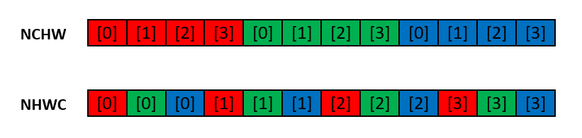
I will swap to “channels last” in the VggNet model and inputs for both training and validation.
model = model.to(device, memory_format=torch.channels_last)
input = input.to(device, memory_format=torch.channels_last)
I implemented these optimizations incrementally and measured the one-epoch training time for a 256 batch for Vgg16 using an NVIDIA GeForce RTX 3090. From this, I will estimate the training time required for 100 epochs (ignoring validation time and other factors). The results are presented in the table below:
| Configuration (cummul.) | Epoch Runtime [min] | Est. Training [hour] | Improvement [%] |
|---|---|---|---|
| CPU | 6400 | 10667 | - |
| GPU | 1000 | 1667 | 540 |
| Workers, pin. etc. | 90 | 150 | 1011 |
| AMP | 55 | 92 | 64 |
| cuDNN | 48 | 80 | 15 |
| Compiled | 38 | 63 | 26 |
| Memory last | 38 | 63 | 0 |
Finally, I ran the fully optimized code on an NVIDIA GeForce RTX 4090, which reduced the per-epoch runtime to around 20 minutes. This means the entire training could be completed in less than 2 days. This was the option selected to move forward with the training.
Training VGGNet and Results
The first decision was which VGGNet configuration to train. According to the results from the original paper, the error rate difference between the deepest and top-performing configurations, VGG16 and VGG19, is less than 0.1% across all testing configurations. In contrast, the error rate difference between configuration B (VGG13) and D (VGG16) is 1.7%. For this reason, I chose to train VGG16 using dense evaluation during testing as a trade-off between accuracy and computational demands.
The training was set up using the exact same hyperparameters, optimizer, and loss function as described in the original paper. As with training AlexNet, the optimizer settings from the original paper will only work if the input has not been rescaled to 1, which in PyTorch means not using transforms.ToTensor. The entire code and output from the training can be found in this repository.
Rather than using my personal (and humble) laptop, the training was conducted on the cloud using RunPod with an NVIDIA GeForce RTX 4090, 24 GB VRAM, 30 GB of RAM, and 6 vCPUs. Personally, I cannot recommend this service enough, as it allows you to access state-of-the-art resources with very little upfront investment. Once you have run the compute-heavy part on the cloud, you can download the model and continue locally.
It took slightly less than two days to train for 100 epochs, during which the learning rate was reduced by a factor of 10 every 30 iterations.
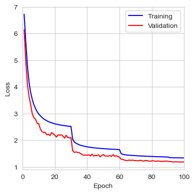
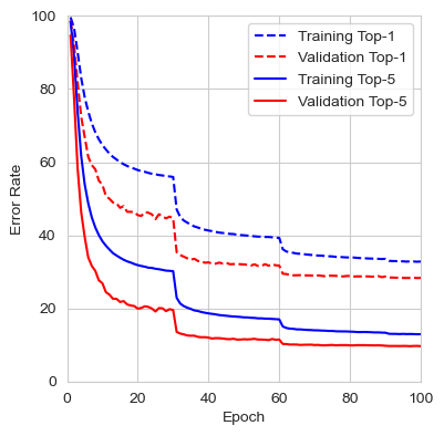
The figure below shows the loss, top-1 error rate, and top-5 error rate over the course of the 100 training epochs. We can observe that the validation set consistently provided lower error rates than the training set. This suggests that by evaluating the input image at different scales and averaging the results, the network finds it easier to identify the correct class. It’s also worth mentioning that during evaluation, the input image is not cropped, so the network has access to the full image with the entire context, which likely contributes to the better performance compared to training. It would be interesting to compare this error rate to that of center-cropped 227x227 images, as done during training.
The results from the last iteration are presented below. In comparison, the authors reported an error rate for VGG16 with multiscale training and dense evaluation of 24.8% for top-1 and 7.5% for top-5, which is lower than the error rate obtained during this training. For the PyTorch VGG16 implementation, the top-1 and top-5 error rates are 28.41% and 9.62%, respectively. These results are much closer to my findings, although it is unclear what testing method the authors used. It is likely that they employed a 224x224 center crop using the fully connected classifier.
| Metric | Train | Validation |
|---|---|---|
| Loss | 1.3405 | 1.1878 |
| Top-1 Error | 32.81% | 28.33% |
| Top-5 Error | 12.93% | 9.66% |
Comparison to AlexNet
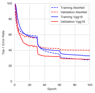
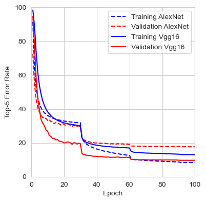
The table below shows the performance comparison between VGG16 and AlexNet after training both from scratch. We can observe that the top-5 error rate on the validation set is approximately 8% better for VGG16. It is also interesting to note that AlexNet’s training error is much lower than its validation error, which could indicate early overfitting. In contrast, VGG16 demonstrates the opposite behavior, with a validation error rate lower than the training error.
| Model | Dataset | Loss | Top-1 Error | Top-5 Error |
|---|---|---|---|---|
| AlexNet | Train | 1.0401 | 27.67% | 8.39% |
| Validation | 1.7083 | 39.93% | 17.73% | |
| VGG16 | Train | 1.3405 | 32.81% | 12.93% |
| Validation | 1.1878 | 28.33% | 9.66% |
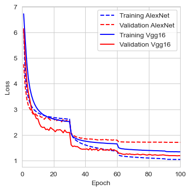
The graphs below show the evolution of the loss, top-1 error rate, and top-5 error rate for both the training and validation sets of AlexNet and VGG16.
Comments
No comments yet.