Implementing AlexNet from Scratch Using PyTorch
Posted on 1/24/2025
-
Last edited on 1/31/2025
This post follows up on ‘Understanding Alexnet’, in which I dived deep into the original paper ImageNet Classification with Deep Convolutional Neural Networks to understand its relevance in the fields of computer vision and machine learning. We also looked at other technical aspects such as data processing, architecture, and results the authors obtained. In this article, I will implement the AlexNet architecture using Pytorch, preprocess the data following the indications from the original paper, implement the appropriate PyTorch transformations, create the learning loops and, finally, train the network, and compare the results with the ones presented by the authors.
Implementing AlexNet’s Architecture
In Pytorch we can create our custom architectures by inheriting from nn.Module, pytorch’s base class for all neural networks. Every neural network will include the following parts:
__init__where the layers are initializedforwardwhere a forward pass is implemented using the previously initialized layers. Note that PyTorch has an automatic differentiation engine that avoids having to implement the gradients ourselves, a complex and error-prone process. This will make it even easier to implement the architecture.
In Python, we have to use the super function in order to make the child class inherit all the methods and properties of the parent. This function calls the parent class __init__ at instantiation, which will allow to use the methods and properties from the parent class. As we want our model class to inherit from nn.Module, we will start the __init__ function with
super(AlexNet, self).__init__()To have all the layers required to build AlexNet, we will need to initialize the following elements. I will refer to the PyTorch documentation as this is the best way to learn about the arguments and details of each element.
- Convolutional layer. Note that the input height and width (spatial dimensions) are not given as parameters to the convolutional layer. We only define the number of input channels (e.g., 3 for an RGB image), the number of kernels (output channels), and other convolutional parameters such as kernel size, stride, and padding. This means that the shape of the output of this layer will depend on the input size used, along with all the defined parameters. I recommend using this ConvNet Output Shape calculatorto keep count of the expected output after each operation. This can be very helpful for debugging and is necessary for defining the number of inputs in the fully connected layer later on.
conv = nn.Conv2d(in_channels, out_channels, kernel_size, stride=1, padding=0)- ReLu You can set
inplace=Trueso that the function modifies the input directly without allocating any additional output, which will save memory during training and testing. Note that in some cases when the original values are needed usinginplace=Truewould cause an error during the automatic differentiation.
relu = nn.ReLU(inplace=True)pool = nn.MaxPool2d(kernel_size, stride=None)- Local response normalization Note that there is a small difference between the formulation in the original paper and PyTorch, as in the paper is not divided by . The settings used later on already account for this difference.
lrn = nn.LocalResponseNorm(size, alpha=0.0001, beta=0.75, k=1.0)- Fully connected layer. Note that
out_featuresis the number of neurons in the fully connected, whilein_featuresis the number of neurons in the previous layer.
fc1 = nn.Linear(in_features, out_features)dropout = nn.Dropout(p=0.5, inplace=False)- Flatten/View: Whenever we need to transition from a convolutional layer to a fully connected layer, we must reshape the tensor into an array. In PyTorch, this can be done using either
flattenorview. Theflattenfunction is essentially an alias for a commonly used case of the more generalviewfunction.
Usingtorch.flatten(x, 1)flattens all dimensions except for the first one, which represents the batch size. The equivalent operation usingviewwould bex.view(x.size(0), -1).
Once we have defined each layer as a class variable, we can also initialize their weights and biases to match those indicated in the original paper.
The weights, which are to be initialized by sampling from a normal distribution, can be set using nn.init.normal_(layer.weight, mean=0.0, std=1.0). The biases can be initialized to a specific value using nn.init.constant_(layer.bias, val).
Note that even though the last activation function should be softmax, I will not include it in the AlexNet architecture. This is because the cross-entropy loss function in PyTorch already includes a softmax at the beginning.
With all these elements, we can then construct our AlexNet convolutional neural network using PyTorch.
import torch
import torch.nn as nn

class AlexNet(torch.nn.Module):
    def __init__(self, num_classes=1000):
        super(AlexNet, self).__init__()
        # Convolutional layers
        self.conv1 = nn.Conv2d(3, 96, 11, stride=4)
        self.conv2 = nn.Conv2d(96, 256, 5, padding=2)
        self.conv3 = nn.Conv2d(256, 384, 3, padding=1)
        self.conv4 = nn.Conv2d(384, 384, 3, padding=1)
        self.conv5 = nn.Conv2d(384, 256, 3, padding=1)

        # Fully connected layers
        self.fc1 = nn.Linear(9216, 4096)
        self.fc2 = nn.Linear(4096, 4096)
        self.fc3 = nn.Linear(4096, num_classes)

        # Initializatin of the weights
        nn.init.normal_(self.conv1.weight, mean=0.0, std=0.01)
        nn.init.normal_(self.conv2.weight, mean=0.0, std=0.01)
        nn.init.normal_(self.conv3.weight, mean=0.0, std=0.01)
        nn.init.normal_(self.conv4.weight, mean=0.0, std=0.01)
        nn.init.normal_(self.conv5.weight, mean=0.0, std=0.01)
        nn.init.normal_(self.fc1.weight, mean=0.0, std=0.01)
        nn.init.normal_(self.fc2.weight, mean=0.0, std=0.01)
        nn.init.normal_(self.fc3.weight, mean=0.0, std=0.01)

        # Initializatin of the bias
        nn.init.constant_(self.conv2.bias, 1.0)
        nn.init.constant_(self.conv4.bias, 1.0)
        nn.init.constant_(self.conv5.bias, 1.0)
        nn.init.constant_(self.conv1.bias, 0.0)
        nn.init.constant_(self.conv3.bias, 0.0)
        nn.init.constant_(self.fc1.bias, 0.0)
        nn.init.constant_(self.fc2.bias, 0.0)
        nn.init.constant_(self.fc3.bias, 0.0)

        # The definition of alpha in the paper and pytorch are slightly different
        self.lrn = nn.LocalResponseNorm(size=5, alpha=5e-4, beta=0.75, k=2.0)
        self.relu = nn.ReLU(inplace=True)
        self.pool = nn.MaxPool2d(kernel_size=3, stride=2)
        self.dropout = nn.Dropout(p=0.5)

    def forward(self, x):
        # Conv1 -> ReLU -> Pool -> LRN
        x = self.conv1(x)
        x = self.relu(x)
        x = self.lrn(x)
        x = self.pool(x)

        # Conv2 -> ReLU -> Pool -> LRN
        x = self.conv2(x)
        x = self.relu(x)
        x = self.lrn(x)
        x = self.pool(x)

        # Conv3 -> ReLU
        x = self.conv3(x)
        x = self.relu(x)

        # Conv4 -> ReLU
        x = self.conv4(x)
        x = self.relu(x)

        # Conv5 -> ReLU -> Pool
        x = self.conv5(x)
        x = self.relu(x)
        x = self.pool(x)

        # Flatten
        x = torch.flatten(x, 1)

        # FC1 -> ReLU -> Dropout
        x = self.fc1(x)
        x = self.relu(x)
        x = self.dropout(x)

        # FC2 -> ReLU -> Dropout
        x = self.fc2(x)
        x = self.relu(x)
        x = self.dropout(x)

        # FC3
        x = self.fc3(x)
        return x
Once the model class is defined, we can instantiate it to work with it. We can also use the torchsummary package to obtain a complete summary of our model’s layers, trainable parameters, output dimensions, and memory utilization. Note that we must also provide the batch size as an input to the summary function.
from torchsummary import summary
# Instantiate model
alexnet = AlexNet(1000)
# Get complete summary of AlexNet
summary(alexnet, (3, 227, 227), batch_size=128)
which produces the following output
----------------------------------------------------------------
        Layer (type)               Output Shape         Param #
================================================================
            Conv2d-1          [128, 96, 55, 55]          34,944
              ReLU-2          [128, 96, 55, 55]               0
 LocalResponseNorm-3          [128, 96, 55, 55]               0
         MaxPool2d-4          [128, 96, 27, 27]               0
            Conv2d-5         [128, 256, 27, 27]         614,656
              ReLU-6         [128, 256, 27, 27]               0
 LocalResponseNorm-7         [128, 256, 27, 27]               0
         MaxPool2d-8         [128, 256, 13, 13]               0
            Conv2d-9         [128, 384, 13, 13]         885,120
             ReLU-10         [128, 384, 13, 13]               0
           Conv2d-11         [128, 384, 13, 13]       1,327,488
             ReLU-12         [128, 384, 13, 13]               0
           Conv2d-13         [128, 256, 13, 13]         884,992
             ReLU-14         [128, 256, 13, 13]               0
        MaxPool2d-15           [128, 256, 6, 6]               0
           Linear-16                [128, 4096]      37,752,832
             ReLU-17                [128, 4096]               0
          Dropout-18                [128, 4096]               0
           Linear-19                [128, 4096]      16,781,312
             ReLU-20                [128, 4096]               0
          Dropout-21                [128, 4096]               0
           Linear-22                [128, 1000]       4,097,000
================================================================
Total params: 62,378,344
Trainable params: 62,378,344
Non-trainable params: 0
----------------------------------------------------------------
Input size (MB): 75.48
Forward/backward pass size (MB): 1880.10
Params size (MB): 237.95
Estimated Total Size (MB): 2193.54
----------------------------------------------------------------
We can see useful data such that the model contains 62,378,344 trainable parameters, the output shape after each layer that we have already computed using the ConvNet Output Shape calculator. We can also preview that each input image takes 73 MB, that saving the model parameters will take 238 MB of disk space, and that the total estimated size is 2.2 GB.
Data Processing
In this section, I will differentiate between two types of data processing: the processing conducted before the training (or preprocessing) and the processing happening during the training phase.
Preprocessing
Database cropping
As we saw in Understanding AlexNet, the ImageNet image size can vary greatly (ranging from the smallest image 20x17 to the largest 7056x4488), which is the reason why the original dataset is so heavy (147 GB!). For that reason, a preliminary step I will take is to transform the original dataset with variable image sizes into one in which all images are 256x256 RGB images.
For that, we will make use of PyTorch’s torchvision library, which contains the most common transformations for computer vision. We will create a new transformation by composing two torchvision-included transformations: Resize and CenterCrop.
import torchvision.transforms as transforms

transform = transforms.Compose([
    # Rescale the image so that the shorter size is of length 256
    transforms.Resize(256),
    # Crop out the central 256x256 path
    transforms.CenterCrop(256),
])
Once the transformation is defined, it can be applied by simply calling it with an image as the argument. The cropping process was done asynchronously to speed it up, and the final function implementation can be found here. After processing the entire dataset, its disk size was reduced from 147 GB to 15 GB.
Mean extraction
After explaining that images will be cropped to be 256x256 RGB images, the original paper says:
We did not pre-process the images in any other way, except for subtracting the mean activity over the training set from each pixel.
A common practice among practitioners working with ImageNet is to normalize the input using mean=[0.485, 0.456, 0.406] and std=[0.229, 0.224, 0.225]. I think I tracked the origin of these values to this commit in 2016 from the PyTorch implementation of ResNet 1, where a comment above the line states that the values were computed from a random subset of ImageNet training images.
For this implementation of AlexNet, I will go through the entire (cropped) training dataset and compute the pixel mean value for each channel, which will be subtracted later on. The specific code used to compute the mean can be found in this repository, together with the resulting matrix mean matrix of shape 256x256x3.
Processing
As explained in Understanding AlexNet, several data augmentation techniques were required to avoid overfitting of the 60 million parameters. For this implementation, all these techniques were implemented as closely as described in the original paper:
- To Tensor: So far we worked with the image object (PIL image), in order to be able to input it to the neural network we have to transorm it into a tensor. The transformation
transforms.ToTensorconverts from a PIL image into a tensor and scales it between [0, 1], however this is not what was done in the original implementation, and if done it will have secondary effects in convergence and hyperparameter selection. For that reason the following function was used rather thantransforms.ToTensor. Note that the order HxWxC is also changed to CxHxW.
def toTensorNoScaling(x):
return torch.from_numpy(np.array(x).transpose(2, 0, 1))- PCA Color Augmentation: I wrote an implementation of PCA Augmentation using the description in the paper and using this repository as a basis. The image is not normalized before computing the eigenvalues, as I suspect it was done origianlly for AlexNet.
def PCAColorAugmentation(img, std=0.1, eps=1e-6):
# Convert PIL image to numpy array
img = np.array(img)
# Original shape (H, W, C)
img_shape = img.shape
# Flatten to (H*W, 3) for RGB channels
img_flat = img.reshape(-1, 3)
# Compute covariance matrix between channels (3x3)
img_cov = np.cov(img_flat, rowvar=False)
# Get eigenvalues and eigenvectors (sorted in ascending order)
eig_vals, eig_vecs = np.linalg.eigh(img_cov)
# Reorder in descending order
eig_vals = eig_vals[::-1]
eig_vecs = eig_vecs[:, ::-1]
# For numerical stability
eig_vals = np.maximum(eig_vals, eps)
# Generate random alphas
alpha = np.random.normal(0, std, 3)
# Compute correction using sqrt of eigenvalues
correction = eig_vecs @ (alpha * np.sqrt(eig_vals))
# Reshape correction
correction = correction.reshape(1, 3)
# Apply correction and clip values
new_img_flat = img_flat + correction
new_img_flat = np.clip(new_img_flat, 0, 255).astype(np.float32)
# Reshape to original dimensions and transpose to CxHxW
new_img = new_img_flat.reshape(img_shape).transpose(2, 0, 1)
# Transform to tensor
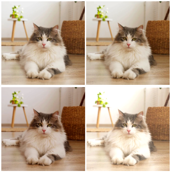
return torch.from_numpy(new_img) I verified this by testing with different images and corrections. For the standard deviation values proposed in the paper (0.1), the color changes are subtle (see the image below). More noticeable changes can be achieved with standard deviation values between 0.3-0.5.
- Mean Subtraction: By using the lambda transformation, we can apply custom functions to the images. I used lambda to apply the transformation to tensor, PCA Color Augmentation, and the per-pixel mean subtraction
x - mean_pixels, already computed. Note that the definition of the function to be used in the lambda transformation should not be a lambda function itself, otherwise, this will raise an error later on. - Random Crop, Horizontal Flip, and Five Crop: PyTorch includes native transformations to perform random crops of a given size, random horizontal flips, and five crops (corners and center).
Finally, all these individual transformations were combined using transforms.Compose. Two different transformations were created: one for training, which includes random transformations for data augmentation, and one for testing, which includes the five-crop transformation and removes random transformations to ensure determinism.
transform_train = transforms.Compose([
    # Apply PCA color transformation and to tensor
    transforms.Lambda(PCAColorAugmentation),
    # Remove mean
    transforms.Lambda(meanSubstraction),
    # 227x227 random crop
    transforms.RandomCrop(227),
    # Horizontal reflection with p=0.5
    transforms.RandomHorizontalFlip(p=0.5),
])

transform_val = transforms.Compose([
    # Transform to tensor without scaling
    transforms.Lambda(toTensorNoScaling),
    # Remove mean
    transforms.Lambda(meanSubstraction),
    # 227x227 corners and center crop
    transforms.FiveCrop(227),
])
Dataset Handling
Preparing a dataset in PyTorch consists of two steps:
- Loading the dataset: This is done via the
torch.utils.data.Datasetclass. PyTorch includes interfaces for the most common datasets, and some can even be downloaded using this interface. Custom datasets can also be defined. In our case, PyTorch already contains the interface for ImageNet, although the data has to be downloaded manually. It’s at this point that we include the transformations that will be applied to each image, as it is theDatasetclass that implements the__getitem__method.
# Load traning and validation data
training_data = torchvision.datasets.ImageNet(filepath, split='train', transform=transform)
validation_data = torchvision.datasets.ImageNet(filepath, split='val', transform=transform)- Create a DataLoader using the dataset: This is done using
torch.utils.data.DataLoader. DataLoaders are iterables over the dataset, allowing for single or multi-process loading, customizing the order, the creation of batches, and memory pinning. Intially, the batch size chosen was 128, as in the original paper.
# Create dataloaders
training_dataloader = torch.utils.data.DataLoader(
    training_data,
    batch_size=128,
    shuffle=True,
    num_workers=0,
    prefetch_factor=None,
    persistent_workers=False,
    pin_memory=False
)

validation_dataloader = torch.utils.data.DataLoader(
    validation_data,
    batch_size=128,
    shuffle=False,  # not needed
    num_workers=0,
    prefetch_factor=None,
    persistent_workers=False,
    pin_memory=False
)
Creating training loop
Implementing a basic training loop in PyTorch is fairly simple. First we need to iterate over the training DataLoader. Each time we iterate over it it will provide a tuple containing: the inputs, a tensor of shape 128x3x227x227; and the associated labels, an array with 128 elements. You check this by writing input, labels = next(iter(dataloader)).
The forward pass is simply done by calling the model with the inputs as an arguments. Then, we can evaluate the loss of the network by calling the instance of the loss function, in our case loss = torch.nn.CrossEntropyLoss(). Below there is an example of a basic training loop.
for input, labels in training_dataloader:
  # Forward pass
  outputs = model(inputs)
  loss = loss_fn(outputs, labels)

  # Backward pass and optimize
  optimizer.zero_grad()
  loss.backward()
  optimizer.step()
For the backward pass, loss.backward() computes the gradient for all tensors in the model, and optimizer.step() updates the weights and biases based on the stored gradient using the selected optimizer. In our case, I used stochastic gradient descent with the hyperparameters as indicated in the paper.
optimizer = torch.optim.SGD(alexnet.parameters(), lr=0.0001, momentum=0.9, weight_decay=0.0005)Bear in mind that by default, PyTorch accumulates gradients, so we need to manually reset them to zero by calling optimizer.zero_grad() before computing new gradients. Accumulating gradients can be useful nonetheless for training RNNs, or when using gradient accumulation when limited GPU memory is available.
Below is a slightly more sophisticated function used to train by iterating once over the entire dataset, also known as an epoch.
def train_one_epoch(epoch_index, writer, model, training_dataloader, optimizer, loss_fn, device):
    """
    Trains AlexNet for one epoch, tracking loss, top-1 and top-5 error rates.

    Args:
        epoch_index: Current epoch number
        writer: TensorBoard writer object
        model: AlexNet model instance
        training_dataloader: PyTorch dataloader for training data
        optimizer: SGD optimizer instance
        loss_fn: CrossEntropyLoss instance
        device: Device to train on (cuda/cpu)

    Returns:
        tuple: (average_loss, average_top1_error, average_top5_error)
    """
    total_loss = 0.0
    running_loss = 0.0
    total_top1_error = 0.0
    total_top5_error = 0.0
    running_top1_error = 0.0
    running_top5_error = 0.0

    # Ensure model is in training mode
    model.train()

    for i, data in enumerate(tqdm(training_dataloader)):
        inputs, labels = data
        inputs = inputs.to(device)
        labels = labels.to(device)

        # Forward pass
        outputs = model(inputs)
        loss = loss_fn(outputs, labels)

        # Backward pass and optimize
        optimizer.zero_grad()
        loss.backward()
        optimizer.step()

        # Calculate top-1 and top-5 error rates
        _, top5_preds = outputs.topk(5, dim=1, largest=True, sorted=True)
        correct_top1 = top5_preds[:, 0] == labels
        correct_top5 = top5_preds.eq(labels.view(-1, 1)).sum(dim=1) > 0
        top1_error = 1 - correct_top1.sum().item() / labels.size(0)
        top5_error = 1 - correct_top5.sum().item() / labels.size(0)

        # Update running statistics
        running_loss += loss.item()
        running_top1_error += top1_error
        running_top5_error += top5_error

        # Update total statistics
        total_loss += loss.item()
        total_top1_error += top1_error
        total_top5_error += top5_error

        # Log every 1000 batches
        if i % 1000 == 999:
            avg_running_loss = running_loss / 1000
            avg_top1_error = 100.0 * running_top1_error / 1000
            avg_top5_error = 100.0 * running_top5_error / 1000

            # Log to TensorBoard
            tb_x = epoch_index * len(training_dataloader) + i + 1
            writer.add_scalar('Loss/train_step', avg_running_loss, tb_x)
            writer.add_scalar('Top-1 error/train_step', avg_top1_error, tb_x)
            writer.add_scalar('Top-5 error/train_step', avg_top5_error, tb_x)

            print(f'  Batch {tb_x} Loss: {avg_running_loss:.4f} Top-1 error rate: {avg_top1_error:.2f}% Top-5 error rate: {avg_top5_error:.2f}%')

            running_loss = 0.0
            running_top1_error = 0.0
            running_top5_error = 0.0

    # Calculate epoch-level metrics
    avg_epoch_loss = total_loss / len(training_dataloader)
    avg_top1_error = 100.0 * total_top1_error / len(training_dataloader)
    avg_top5_error = 100.0 * total_top5_error / len(training_dataloader)

return avg_epoch_loss, avg_top1_error, avg_top5_errormodel.train()is used to tell PyTorch that we are about to train the model. In our case, this means that dropout will be active.- One handy tool that has transitioned from TensorFlow to PyTorch is TensorBoard’s
SummaryWriter, which allows us to visualize metrics in a built-in interface during training using theadd_scalarmethod.SummaryWriteralso supports many other visualizations, such as model and batch visualizations.
from torch.utils.tensorboard import SummaryWriter

writer = SummaryWriter()
writer.add_scalar(tag, scalar_value, global_step=None)- Every 1000 batches, the function prints the loss value along with the top-1 and top-5 error rates, similar to the evaluation method used in the original paper. The same data is also stored using TensorBoard’s writer.
A similar function, validate_one_epoch, was implemented, with the only difference being that the model is set to evaluation mode by toggling model.eval() and using with torch.no_grad(): to disable gradient computation, as it is not needed during this phase. Refer to the repository for more details.
Finally, the complete training loop was created by iterating over train_one_epoch and validate_one_epoch for epochs. Instead of using a scheduler to reduce the learning rate when the average validation loss plateaus, as done in the original AlexNet, I chose to decrease the learning rate by a factor of 10 every 30 iterations, ensuring it has decreasesd three times over 90 iterations.
scheduler = torch.optim.lr_scheduler.StepLR(optimizer, step_size=30, gamma=0.1)The model with the best average validation loss is saved as a checkpoint in case the training stops or crashes for any reason.
Speeding up training
Using the code given up to this point, we could already run and train the network by executing train_one_epoch successively. However, there is a problem, this naive implementation is painfully slow. Running it on my old humble gaming laptop with 8GB of RAM and an NVIDIA GTX 1050 4GB GPU would take 44 hours (!) to complete just one epoch.
If we need 90 epochs to train AlexNet, as stated in the original paper, this would amount to 3960 hours or 165 days (!!!) to complete training.
In this section, I will go through the different approaches I tried to speed up training, which mainly involve applying some of the techniques from this Reddit post.
- CPU to GPU: Using the GPU instead of the CPU for training is, obviously, the first improvement. We can move a model or variable to the GPU using
.to(device), wheredeviceis set to the GPU if available, otherwise it will be CPU. By transferring both the model and data to the GPU, the training time for one epoch is reduced from 44 hours to just 7 hours.
To ensure compatibility across different machines, we can definedeviceas follows:
device = torch.device('cuda' if torch.cuda.is_available() else 'cpu')- Model Compilation: PyTorch provides an easy way to compile models for faster training. Compiling a model is as simple as running
torch.compile(model). However, when I tried to compile my AlexNet, I encountered an error stating that PyTorch no longer supports this GPU because it is too old, which means that this optimization had to be ruled out. - Automatic Mixed Precision (AMP): PyTorch includes a mechanism to automatically switch from FP32 (full-precision floating-point format) to FP16 (half-precision floating-point format), allowing certain operations to run faster without significant loss of accuracy. However, in my tests, I did not observe a significant reduction in epoch runtime, so I chose not to use it.
- Multiple Workers and Pinned Memory: Three important parameters of
torch.utils.data.DataLoadercan help speed up data loading:num_workers: Allows parallelizing data loading by specifying the number of worker processes. We can determine the number of available CPU cores in Python usingos.cpu_count().pin_memory: Enables copying tensors into pinned memory before returning them, improving transfer speed to the GPU.prefetch_factor: Enables workers to load batches in advance, reducing waiting time. Note that this value indicates the batches loaded in advance per worker.
By setting num_workers=4, prefetch_factor=4, persistent_workers=True, and pin_memory=True, the time to train one epoch was reduced from 7 hours to 1 hour and 40 minutes.
- Turning on cuDNN: By setting
torch.backends.cudnn.benchmark = True, the cuDNN autotuner benchmarks different convolution computation methods and selects the fastest one. However, after enabling it, the training quickly crashed due to insufficient memory, so I chose not to use it. - Increasing the Batch Size: I tried to double the batch size to 256, but the training crashed again due to memory limitations.
- Gradient Accumulation: I tested gradient accumulation, but I decided not to use it to stay closer to the original paper’s training methodology.
The table below summarizes the methods tested to speed up the training.
| Method | Implemented | Time [hours] |
|---|---|---|
| Naive | No | 44 |
| CPU to GPU | Yes | 7 |
| Model Compilation | Unavailable | |
| Automatic Mixed Precision | No | 6.5 |
| Multiple workers & Pinned memory | Yes | 1.75 |
| Turning on cudNN | Crashed | - |
| Incrementing the batch size | Crashed | - |
| Gradient Accumualtion | No | - |
| Update Using RTX 3090 | Yes | 0.3 |
Finally, the runtime for one epoch ended up being 1.75 hours, meaning that training the final network will take approximately 158 hours or 6.5 days. This is in the same order of magnitude as the time it took to train the original AlexNet.
Update: Due to the long computing times while debugging I decided to use RunPod to be able to iterate faster. The extra RAM and RTX 3090 allowed me to reduce the epoch time to 11 minutes by increasing the batch and number of workers.
Training AlexNet and Results
And finally, the moment of truth had arrived, the moment of training my first deep convolutional neural network on a very large dataset like ImageNet.
The training lasted for 100 epochs, taking approximately 25 hours. The entire code and training output can be found in the repository. The learning rate started at 0.01 and was reduced by a factor of 10 every 30 epochs.
The figures below show the loss, top-1 error rate, and top-5 error rate throughout training. During the first 30 epochs, the training and validation sets showed similar behaviors. However, after the learning rate was reduced, the model started to overfit more on the training data, although some improvement was still observed in the validation set. The model did not reach a point where a decrease in training loss produced an increase in validation loss, but at the end of the training, improvements in the validation set had become marginal.
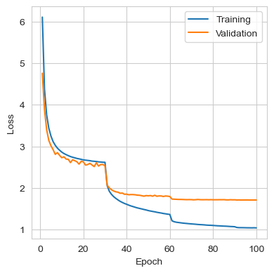
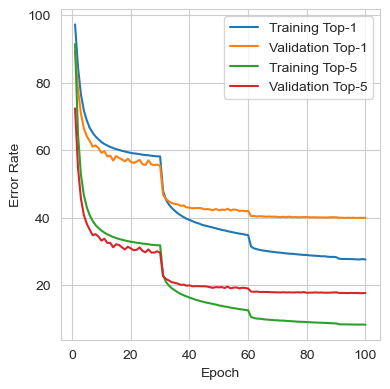
The metrics from the best iteration are shown in the table below. It can be seen that the performance closely matches the results reported in the original paper, where a single standard AlexNet achieved top-1 and top-5 validation error rates of 40.7% and 18.2%, respectively.
| Metric | Train | Validation |
|---|---|---|
| Loss | 1.0401 | 1.7083 |
| Top-1 Error | 27.67% | 39.93% |
| Top-5 Error | 8.39% | 17.73% |
Lessons Learnt
During the setup and debugging of the AlexNet training process, there were, as always, some challenges. I would like to highlight some of the lessons learned during this process:
- Working with ImageNet is hard. My recommendation is to avoid trying to work with it unless you are using an SSD, as the computational time required to load and process the 1,281,167 training images can become extremely lengthy. Once you switch to the cropped version of the dataset, things become much more manageable.
- Spending time discovering which optimization techniques to use for speeding up a single epoch of training is essential, as even small improvements will scale up by around three orders of magnitude for the training.
- There is one big inappreciated difference between the modern implementations of AlexNet that I found online and the original one. Since most of the modern implementations use
transforms.ToTensorby default. They don’t realize that the scaling form 0-255 to 0-1 influences the entire scaling of the problem. This causes that when trying to train AlexNet with the optimizer and hyperparameters from the paper, the network does not converge. This happended to myself at the beginning, when I used, unware, the [0-1] normalization. And I found examples of this in this post and also this repository. They were uncapable of getting SGD to move, and ended up using Adam with a learning rate of 0.0001. Nonetheless, if the inputs are not normalized, SGD using a learning rate of 0.01 and the initial weights indicated will converge. Moreover, I also found the optimizer to converge without problems when using inputs where the mean was not substracted. - There is one big inappreciated difference between the modern implementations of AlexNet that I found online and the original one. Since most modern implementations use
transforms.ToTensorby default, they don’t realize that rescaling from 0-255 to 0-1 influences the entire the problem, also in other areas. This causes that when trying to train AlexNet with the optimizer and hyperparameters from the paper, the network does not converge. I encountered this issue myself at the beginning when I unknowingly was using the [0-1] normalization and I also found examples of this in this post and this repository, where they were unable to get SGD to move in any direction and ended up using Adam with a learning rate of 0.0001.
However, if the inputs are not normalized, then SGD with a learning rate of 0.01 and the initial weights from the paper will converge. Additionally, I also found that the optimizer converged without issues when using inputs where the mean was not subtracted as well.
Footnotes
-
He, K., Zhang, X., Ren, S., & Sun, J. (2016). Deep residual learning for image recognition. In Proceedings of the IEEE conference on computer vision and pattern recognition (pp. 770-778). ↩
Comments
No comments yet.